
MOTION CAPTURE OF AN ANIMATED SURFACE
VIA SENSORS’ RIBBONS
Surface Reconstruction via Tangential Measurements
Nathalie Sprynski
CEA-LETI, MINATEC Campus, Grenoble, France
Bernard Lacolle, Luc Biard
Laboratoire Jean Kuntzmann, Universit
´
e Joseph Fourier, Grenoble, France
Keywords:
Motion capture, Micro-sensors, Surface reconstruction, Curve reconstruction, Hermite interpolation.
Abstract:
This paper deals with the motion capture of physical surfaces via a curve acquisition device. This device is a
ribbon of sensors, named Ribbon Device, providing tangential measurements, allowing to reconstruct its 3D
shape via an existing geometric method. We focus here on the problem of reconstructing animated surfaces,
from a finite number of curves running on these surfaces, acquired with the Ribbon Device. This network
of spatial curves is organized according a comb structure allowing to adjust these curves with respect to a
reference curve, and then to develop a global C1 reconstruction method based on the mesh of ribbon curves
together with interpolating transversal curves. Precisely, at each time position the surface is computed from
the previous step by an updating process.
1 INTRODUCTION
We are concerned with the reverse engineering prob-
lem of re–constructing animated physical surfaces
from tangential data. These tangential data are pro-
vided by embedded sensors (micro–accelerometers
and micro–magnetometers) along a curve represented
by a ribbon. This problem is not a dual interpola-
tion or approximation problem (Hoschek, 1983) as
the tangential data are not localized in space. Appro-
priate methods for the reconstruction of planar and
spatial curves from such tangential information have
been developed in (Sprynski et al., 2007) and have
been validated by a real-time demonstrator: a ribbon–
like device, denoted Ribbon Device – see Figure 1
– equipped with 32 micro–sensors. See also (Hoshi
and Shinoda, 2008) for a prototype of sensing device,
analogous to a rectangular grid of linear instrumented
segments, providing thus elementary geometry.
The deep novelty of such capture/reconstruction
approaches is to deal with purely orientation data.
Furthermore, notice that all previous related works
only consider static surfaces. We are thus concerned
in this paper with the motion capture of a surface
in deformation from a network of spatial curves run-
ning on the surface, obtained with the Ribbon Device.
Precisely, by placing the Ribbon Device on a physi-
cal surface at regular intervals, the surface is divided
into a system of patches, which can be then filled by
interpolating Coons processes (Coons, 1964; Coons,
1974; Farin, 2002). See also (Peters, 1990; Sarraga,
1987; Shirman and S
´
equin, 1987) for construction
processes of smooth surfaces from given boundary
curve data. The shape of the surface is thus essentially
modeled by these spatial curves forming a character-
istic mesh of the surface.
Applications are countless, ranging from medical
applications (e.g. determining shape and curvature of
the spinal column), to aerodynamic applications (e.g.
acquiring the shape and deformation of a wing).
This document is organized as follows. The sen-
sors, the acquisition tool and the process used for sur-
face capture are detailed in Section 2. Section 3 fo-
cuses on the algorithms developed to solve the prob-
lem, which first consists in reconstructing the ribbon
curves, and then the interpolating surface. Finally,
Section 4 deals with the validation and the implemen-
tation.
421
Sprynski N., Lacolle B. and Biard L..
MOTION CAPTURE OF AN ANIMATED SURFACE VIA SENSORS’ RIBBONS - Surface Reconstruction via Tangential Measurements.
DOI: 10.5220/0003330604210426
In Proceedings of the 1st International Conference on Pervasive and Embedded Computing and Communication Systems (PECCS-2011), pages
421-426
ISBN: 978-989-8425-48-5
Copyright
c
2011 SCITEPRESS (Science and Technology Publications, Lda.)
2 ACQUISITION STEPS
2.1 The Acquisition Tool
What is targeted here is to introduce new kinds of in-
strumented materials. We think for example about
plastic or textile ribbons or surfaces, which will be
equipped with arrays of sensors in order to gain some
new properties. The alliance between instrumented
materials and mathematical algorithms will allow ma-
terials to be able to access some knowledge about
their own shape, introducing what we could call pro-
prioceptive materials. The approach for building such
materials is presented.
2.1.1 Sensors
First step is to provide angular adequate information
for surface computation. For that purpose, the follow-
ing microsensors arre used.
• Microaccelerometers are able to provide the angle
between the sensor and the vertical (as long as the
sensor is quite static).
• Micromagnetometers are able to provide angular
information with the earth magnetic field (when
no magnetic pertubations around them occur).
These sensors have to be combined as a biaxial or a
triaxial way, in order obtain the exact orientation of
the measure point in the space (Fontaine et al., 2003).
Five different measure from sensors are necessary to
have the exact orientation (three accelerometers in a
triaxial organization, and two magnetometers in a bi-
axial way). This study allows the creation of the pro-
totype.
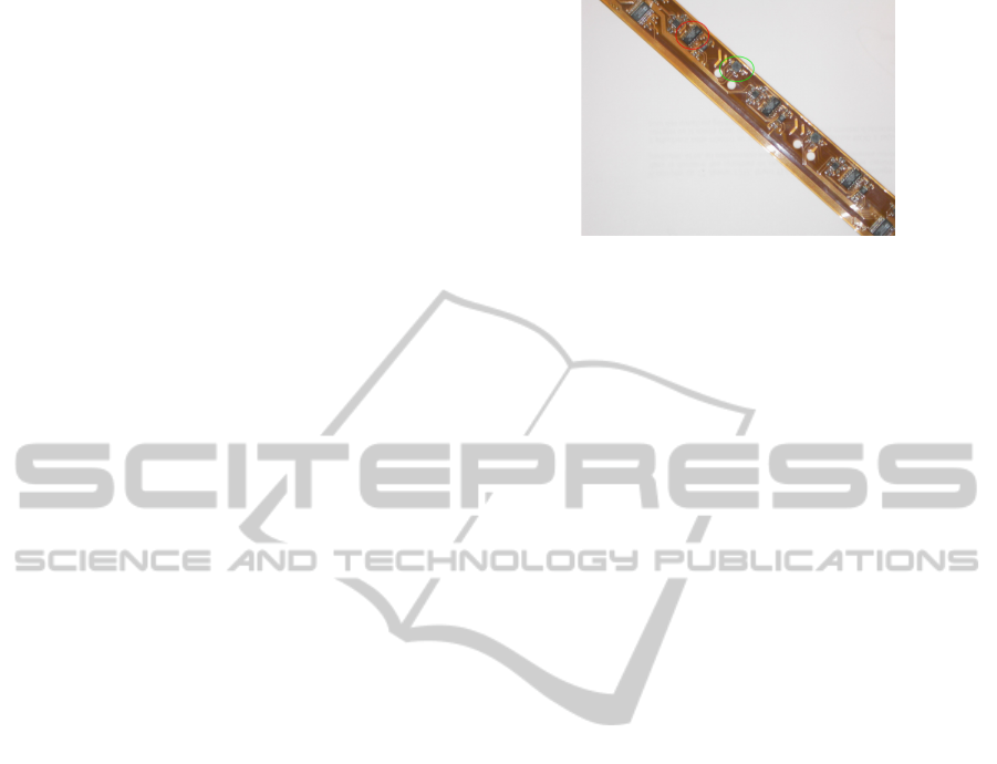
2.1.2 The Ribbon
Our new generation ribbon has been developed with
the considerations above. The ribbon is equipped with
a set of sixteen 3D microaccelerometers, alternating
with a set of sixteen 2D micromagnetometers (AMR
type sensors from Honeywell or similar). They are
mounted on a flexible PCB ribbon. The distance be-
tween the sensors is nearly 25 mm. Such arrangement
of the sensors allows gaining complete tangential in-
formation (not exactly at each sensor location, but for
a set of two adjacent sensors). The sensors are read
via a SPI serial bus, which allows a lot of sensors (see
Figure 1). This ribbon is also easy to use thanks to its
Bluetooth connection to the host computer. Finally, a
software driver has been designed which allows to se-
quentially read all sensor values at different sampling
Figure 1: Ribbon of sensors able to provide 3D tangential
data.
rates. In fact, the current ribbons are essentially proto-
types that have been used for demonstration and val-
idation purpose. Some technological issues are cur-
rently being addressed concerning sensor embedding
in ribbons.
• Connections: we want to connect wires to a pos-
sibly great number of sensors. Solutions already
exist at the die scale, but not at larger scales (up
to meters). Dedicated connection technologies are
currently being studied.
• Reliability: as the ribbon is planned to be flexible,
most existing technologies do not apply. We are
also studying various solutions to get such relia-
bility.
Our final goal is to be able to produce ribbons and sur-
faces embedding possible large sensors areas, while
keeping the advantage of low cost sensors.
2.1.3 The Ribbon Curve
The ribbon described above is able to provide its own
shape. More precisely, methods have been developed
to reconstruct curves via data from the ribbon, the
curve being denoted ribbon curve (see Appendix A).
Data are tangential data at sensors’ positions, and dis-
tances between sensors along the ribbon. Let us no-
tice that we do not have any information concerning
absolute positions of any points of the ribbon, such
that the ribbon curves reconstructed are unique up to
their starting point.
2.2 Surface Acquisition Process
We have to acquire a surface via a ribbon of sensors,
thus we have to reconstruct a surface from a finite
number of ribbon curves laying on it. As it does not
exist an intrinsic parameterization for surfaces (con-
trary to the curves with the arc-length parameter), we
will keep the linear organization of sensors, and the
ribbons are then a natural way to acquire surfaces.
The question is thus as follows : how can we orga-
nize curves on a surface in order to know it ? Two
PECCS 2011 - International Conference on Pervasive and Embedded Computing and Communication Systems
422
kinds of organization appear. The first one is a mesh
of ribbons, where sensors are on the intersections.
The surface is known by two families of curves in
two complementary directions, so that we have a ten-
sorial topology of the surface. This problem is well
posed but this acquisition system is not really easy to
use (how can we put it on non-developable surfaces?
How can we put ribbons to cross exactly on sensors’
positions?). So, in a more general case, we consider a
second acquisition system, which consists in one fam-
ily of ribbons in the same direction.
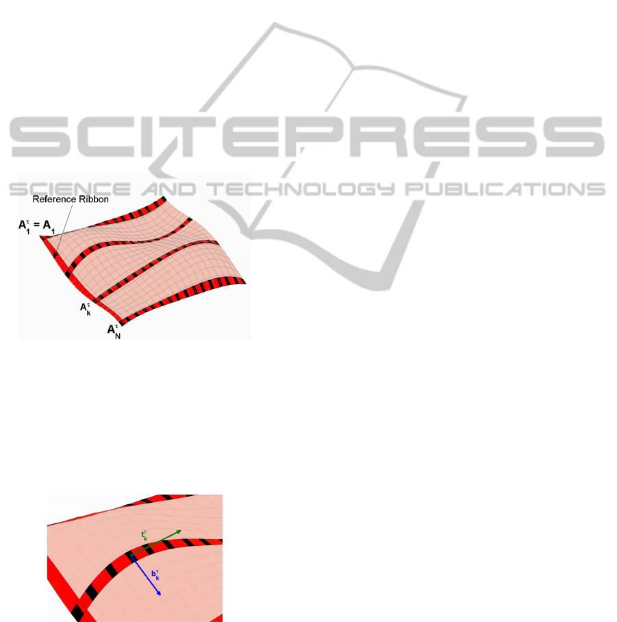
More precisely, we fix ribbons in the same direc-
tion on a mobile surface. Figure 2 shows an exam-
ple of acquisition process with four parallel ribbons
(in red), with sensors represented in black squares.
In that case, ribbon curves are reconstructed inde-
pendently, thus we have to fix their relative position
with each other: we use an additional ribbon in the
transversal direction, denoted reference ribbon link-
ing all starting points A
k
: thus we have a comb struc-
ture of ribbons to acquire a surface.
Figure 2: Surface acquisition process with 4 ribbons.
These ribbons give at each sensors’ point tangen-
tial information (two vectors at sensors’ position: t
τ
k
tangential vector of the ribbon curve, b
τ
k
binormal
vector of the ribbon curve in the tangent plane (ribbon
seen as a surface, equivalent to the surface to acquire
at these points) (see Figure 3).
Figure 3: Tangential data given by sensors : unit tangent
vector t
τ
k
and unit binormal vector b
τ
k
.
When the surface is moving, ribbons are following
the surface deformations. The surface is thus known
via the moving curves laying on it. The figure 5-left
illustrates the process.
The physical surface is then described with the
flow of the tangential constraints (given by sensors
on ribbons), with length constraints along the rib-
bons. The sensors are organized in a comb structure,
with tangential data in both directions, but length con-
straints in only one direction (the ribbon curves direc-
tion).
3 SURFACE RECONSTRUCTION
As the surface acquisition process – with a comb
structure – induces a tensorial structure on the physi-
cal surface, we consider the following reconstruction
strategy.
At each time position :
1- we reconstruct the 3D ribbon curves from sensors
data and length constraints,
2- these ribbon curves are adjusted according the
comb structure,
3- from which we deduce the transversal 3D curves
from sensors’ data, but without any length infor-
mation,
4- finally, the surface is filled by a standard cubic
Coons process.
The main strategy is thus to follow the ani-
mated/deformed ribbons.
Step 1 has been validated in case of static recon-
struction but could be time expensive. So, for real
time reconstruction, the 3D ribbon curves at time po-
sition τ+∆τ are deduced from the 3D ribbon curves at
time position τ by an iterative/minimisation process.
Precisely, Step 1 splits into two phases.
1a- Initialization – At time position τ = 0, the 3D
initial ribbon curves are reconstructed from the
method described in Appendix A.
1b- Iterative step – The 3D ribbon curves at time po-
sition τ + ∆τ are deduced by an updating process
from the tangential data of sensors at time τ + ∆τ
and the sensors’ position at time τ.
Notice that each ribbon curve is reconstructed up
to an arbitrary starting point, in Steps 1a and 1b.
These ribbon curves are then adjusted in Step 2 by
using the reference ribbon curve. Finally, the whole
reconstruction process will produce a C
1
surface.
3.1 Ribbon Curves Reconstruction
As Step-1a is detailed in Appendix A, we now focus
on the iterative Step-1b. Assume we have N + 1 rib-
MOTION CAPTURE OF AN ANIMATED SURFACE VIA SENSORS' RIBBONS - Surface Reconstruction via
Tangential Measurements
423

bons (one of them being the reference ribbon curve),
each of these ribbons being equipped with n + 1 sen-
sors numbered from 0 to n.
Considering any of these ribbons, each segment
ribbon curve r
τ+∆τ
k
(s) between sensor k and sensor
k + 1, at time position τ + ∆τ, is modeled, as a cubic
Hermite curve (see Appendix B)
r
τ+∆τ
k
(t) = H[p
τ+∆τ
k
, p
τ+∆τ
k+1
, t
τ+∆τ
k
, t
τ+∆τ
k+1
;s
k
, s
k+1
](t),
(1)
where :
⋄ points p
τ+∆τ
k
, p
τ+∆τ
k+1
are the unknown positions of
sensors k and k + 1 at time position τ + ∆τ,
⋄ vectors t
τ+∆τ
k
, t
τ+∆τ
k+1
are the (updated) tangential
information along the curve provided by sensors
k and k + 1 at time τ + ∆τ,
⋄ s
k
, s
k+1
are the arc length positions of sensors k
and k + 1 along the ribbon.
Then, the length constraints between sensors along
the ribbon provide additional relations
∫
s
k+1
s
k
∥
d
dt
r
τ+∆τ
k
(t)∥dt = s
k+1
− s
k
, (2)
for k = 0, ..., n − 1 , at each time τ + ∆τ. Expand-
ing these integrals yield non linear constraints. Fur-
thermore, as equations (2) do not have a unique so-
lution, we consider the supplementary minimization
constraints for k = 0, ..., n − 1
min
∫
s
k+1
s
k
∥
d
2
dt
2
r
τ+∆τ
k
(t)∥
2
dt . (3)
Finally, as constraints (2) and (3) allow to de-
termine uniquely one of the two unknown position
points of each segment ribbon curve, the method for
the ribbon curve reconstruction proceeds iteratively as
follows for each curve.
– Choose point p
τ
0
as starting point p
τ+∆τ
0
of the rib-
bon curve.
– For each segment ribbon curve r
τ+∆τ
k
(s), k =
0, ..., n − 1, compute the ending point p
τ+∆τ
k+1
from
relations (1) with the updated vectors t
τ+∆τ
k
, t
τ+∆τ
k+1
,
and the (previously computed) starting point
p
τ+∆τ
k
, from constraints (2) and (3). This mini-
mization step is initialized with the previous point
p
τ
k+1
.
The Hermite definition (1) insures that the recon-
structed ribbon curves will be C
1
. Moreover, the en-
ergy constraint (3) on each segment ribbon curve in-
sures to get a smooth ribbon curve among the family
of curve solutions, i.e., C
1
cubic splines. Notice that
these C
1
splines are not the classical ones as the initial
data are tangent directions instead of 3D points.
3.2 Comb Structure Updating
As each ribbon curve is reconstructed up to an arbi-
trary starting point in the previous steps, we are now
faced to adjust these curves according the reference
ribbon curve.
This step is based on the two following points.
- The reference ribbon curve is reconstructed up to
(the reference) point A
τ
1
= A
1
at each time position
τ, see Figure 2. So that the whole surface will be
reconstructed with respect to that point.
- Then, each “orthogonal” ribbon curve is trans-
lated in order its starting point match with the cor-
responding point A
τ
k
.
3.3 Transversal Curves
At this point, we know at each time position the sen-
sor’s 3D position on each ribbon curve together with
its associated transversal tangential information: the
binormal vector, see Figure 3.
Figure 4: Future physical testing framework device.
Denoting more precisely by p
τ
k, j
the 3D position
of sensor k on the ribbon curve j and by b
τ
k, j
the as-
sociated unit binormal vector, at each time position τ,
we consider the cubic Hermite curve (see Appendix
B) joining sensors k on ribbon curves j and j + 1
x
τ
k, j
(t) (4)
=H[p
τ
k, j
, p
τ
k, j+1
, λ
τ
k, j
b
τ
k, j
, λ
τ
k, j+1
b
τ
k, j+1
;t
j
,t
j+1
](t),
with t
j
= j −1 and where λ
τ
k, j
are positive coefficients
associated with sensor k of the ribbon curve j at time
position τ.
Then, considering the C
1
spline curve x
τ
k
(t), com-
posed of segment curves x
τ
k, j
(t), the following mini-
mization energy
min
∫
N−1
0
∥
d
2
dt
2
x
τ
k
(t)∥
2
dt , (5)
leads to determine unique values for coefficients λ
τ
k, j
,
producing smooth C
1
Hermite interpolating transver-
sal curves.
PECCS 2011 - International Conference on Pervasive and Embedded Computing and Communication Systems
424

Figure 5: Left: animated analytical surface – Right: the reconstructed animated surface.
3.4 Surface Filling
At this point, the physical surface is recon-
structed/modeled by a network of two families of “or-
thogonal” C
1
spline curves meeting at sensors’ posi-
tion, delimiting thus a set of n(N −1) curvilinear rect-
angles.
Each of these curvilinear rectangles is then filled
by a partially bi-cubically blended Coons process
(Coons, 1974), producing a G
1
global surface.
Notice that this whole reconstruction process al-
lows to faster refresh the display of the reconstructed
surface, by only considering the previous network of
“orthogonal” curves as a mesh approximating the sur-
face.
4 CONTROL AND VALIDATION
The validation of such methods requires to compare
the physical deformed surfaces and the reconstructed
shapes at each time position, and clearly, a visual con-
trol is not sufficient. We describe here the experimen-
tal device under development for this purpose.
4.1 Experimental Device
We are currently developing a physical testing frame-
work surface (see Figure 4), animated and controlled
by a mechanical device. The surface motion is ac-
quired by an optical system, providing an external re-
liable control.
By placing ribbons of sensors on this testing
framework surface, according the process described
in Section 2.2, we will acquire a network of animated
spatial curves on this surface, allowing to compare the
reconstructed surface by our process with the “optical
surface” reconstructed from the external acquisition
optical system.
Furthermore, the acquisition process of moving
surfaces is intricate and requires a precise methodol-
ogy. While the surface is moving, the physical ribbon
will not keep an intrinsic position on the surface and
will slip on the surface. Precisely, it is proved that
these ribbons actually follow geodesic curves on the
physical surface. Thus, when the surface is deformed,
the ribbons slip in order to remain a geodesic on the
surface. This is not a blocking point for our method
as we need only distance information of the starting
points of the curves, the ribbons remaining fixed at
the origin.
4.2 Computed Examples
The animated analytical surface described in Fig-
ure 5-left is reconstructed using our process, see Fig-
ure 5-right.
An error is estimated between the animated
analytical model of the surface and the re-
constructed animated surface at some time po-
sition. Precisely, at each time position τ,
the error is computed at sensors’ position as
E(τ) =
100
(n + 1)N L
rib
N
∑
j=1
n
∑
k=0
∥
˜
p
τ
k, j
− p
τ
k, j
∥
where
˜
p
τ
k, j
and p
τ
k, j
are respectively the sensor’s posi-
tion on the physical surface and on the reconstructed
surface, and where L
rib
is the ribbon’s length.
Figure 5 exhibits an example with a mean error
equal to 1.68%, comprised in the interval [1.18, 2.57],
on a sample of 120 time positions.
5 CONCLUSIONS
A strategy for the acquisition of animated surfaces via
a ribbon of sensors has been developed in this paper.
The method is based on a comb structure of the recon-
structed ribbon curves according a reference curve.
MOTION CAPTURE OF AN ANIMATED SURFACE VIA SENSORS' RIBBONS - Surface Reconstruction via
Tangential Measurements
425

This approach allows to adjust the network of the re-
constructed curves running on the surface and to get
a “coherent” mesh interpolating the animated surface
by an updating process from the previous time posi-
tion. The method has been tested on an animated an-
alytical surface.
Then, in order to validate the method in the gen-
eral case of a physical animated surface, a testing
framework surface is under development, so that, per-
formance comparisons with real physical data have
not been realized yet. Anyway, the first experiments
have highlighted some practical difficulties concern-
ing the implementation of the acquisition process. Es-
sentially, we have to ensure a permanent smooth con-
tact between the ribbon and the animated surface. So-
lutions (i.e., smoother and more flexible ribbons,...)
are on progress.
REFERENCES
Coons, S. (1964). Surfaces for computer aided design.
Technical Report, M.I.T.,1964, Available as AD 663
504 from the National Technical Information service,
Springfield, VA 22161.
Coons, S. (1974). Surface patches and b-spline curves.
Computer Aided Geometric Design, In R. Barnhill
and R. Riesenfeld editors, Academic Press.
Farin, G. (2002). Curves and Surfaces for CAGD - Fifth
Edition. Academic Press.
Fontaine, D., David, D., and Caritu, Y. (2003). Sourceless
human body motion capture. In Proc. Smart Objects
Conference (SOC’03).
Hoschek, J. (1983). Dual b
´
ezier curves and surfaces. Com-
puter Aided Geometric Design, North Holland, pages
147–156.
Hoshi, T. and Shinoda, H. (2008). 3d shape measuring
sheet utilizing gravitational and geomagnetic fields. In
Proceeding of the SICE Annual Conference 2008. The
University Electro-Communications, Japan.
Nielson, G. (2004). ν-quaternion splines for the smooth
interpolation of orientations. IEEE Transactions on
visualization and computer graphics, 10(2):224–229.
Peters, J. (1990). Local smooth surface interpolation: A
classification. Computer Aided Geometric Design,
7:191–195.
Sarraga, R. F. (1987). G1 interpolation of generally unre-
stricted cubic b
´
ezier curves. Computer Aided Geomet-
ric Design, 4:23–39.
Shirman, L. A. and S
´
equin, C. H. (1987). Local surface in-
terpolation with b
´
ezier patches. Computer Aided Ge-
ometric Design, 4:279–295.
Sprynski, N., Lacolle, B., David, D., and Biard, L. (2007).
Curve reconstruction via a ribbon of sensors. In Pro-
ceeding of the 14th IEEE International Conference on
Electronics Circuits and Systems. ICECS, Marrakech,
Maroc.
APPENDIX
A: Initial Reconstructed Curves. A 3D curve
C(s) = (x(s), y(s), z(s)), parameterized with respect to
its arc-length s satisfy |C
′
(s)| ≡ 1, so that the deriva-
tive curve C
′
(s) is a curve lying on the unit sphere.
Initial data are unit tangential vectors at points with
assigned arc length parameters. The methodology is
thus as follows.
• First, we interpolate data using cubic splines on
the sphere, leading to the derivative curve C
′
(s).
• Then, by integration we get a solution for C(s).
Cubic splines on the unit sphere (see (Nielson, 2004))
are an extension of the usual B-splines in the euclid-
ian space. The main differences are the following.
⋄ The evaluation of the control polygon of cubic
splines on the spherical space requires to solve a non
linear system through an iterative algorithm.
⋄ The usual De Casteljau algorithm, based on linear
interpolations, has to be replaced by the spherical in-
terpolation
Sler p(a, b, t) =
sin((1 −t)θ)a + sin(tθ)b
sin(θ)
,
where a and b are two unit vectors, θ the angle be-
tween vectors a and b, and t ∈ [0, 1].
It is proved in (Sprynski et al., 2007) that this con-
struction is invariant under rotations and scaling, and
that these spherical splines minimize a combination
of the curvature κ
1
, the torsion κ
2
, and the variations
of the curvature, precisely
min
∫
(κ
′2
1
+ κ
2
1
(κ
′2
1
+ κ
2
2
)),
which gives physical sense to the reconstruction.
B: Cubic Hermite Interpolation. Given spatial
points p
0
and p
1
associated with tangent vectors t
0
and t
1
, together with two parameters α
0
and α
1
(α
0
<
α
1
), there exists a unique cubic spatial parametric
curve r(t) such that
r(α
0
) = p
0
, r(α
1
) = p
1
, r
′
(α
0
) = t
0
, r
′
(α
1
) = t
1
.
Precisely, r(t) is defined by
r(t) = H
0
(
ˆ
t)p
0
+ H
1
(
ˆ
t)p
1
+ (α
1
− α
0
)H
2
(
ˆ
t)t
0
+ (α
1
− α
0
)H
3
(
ˆ
t)t
1
,
with
ˆ
t =
t−α
0
α
1
−α
0
and where functions φ
j
are the cu-
bic Hermite polynomials (Farin, 2002) on the interval
[0, 1], and r(t) and is denoted shortly by
r(t) = H[p
0
, p
1
, t
0
, t
1
;α
0
, α
1
](t).
PECCS 2011 - International Conference on Pervasive and Embedded Computing and Communication Systems
426
