
3D OPTICAL FLOW FROM DOPPLER AND WINDPROFILER
RADAR DATA
Yong Zhang, John L. Barron and Robert E. Mercer
Dept. of Computer Science, The University of Western Ontario, London, N6A 5B7, Ontario, Canada
Keywords:
3D Doppler radial velocity, 3D Windprofiler velocity, 3D Least squares optical flow, 3D Regularized optical
flow, 3D Full velocity field.
Abstract:
We describe an application that combines velocity data from a Windprofiler radar and a NEXRADII Doppler
radar to compute 3D optical flow of moving severe weather. Windprofiler data improves the recovery of the
velocity component in the upwards direction in the optical flow, where Windprofiler data is believed to be
more accurate. We demonstrate this quantitatively using synthetic radar data and qualitatively using real radar
data from Detroit NCDC Doppler and Harrow Windprofiler radars.
1 INTRODUCTION
Doppler radar is an important meteorological obser-
vation tool. To gain knowledge of how storms move
over time, much research has been devoted to re-
trieving 3D full velocity from the observed radial ve-
locity (for example, Lhermitte and Atlas (Lhermitte
and Altas, 1961), Easterbrook (Easterbrook, 1975)
and Waldteufel and Corbin (Waldteufel and Corbin,
1979)). Rather than using the traditional methods pro-
vided by meteorologists, our research group is solving
this problem using the 3D Optical Flow framework
(Barron et al., 2005), which is a technology widely
applied in Computer Vision. In this paper, we “refine”
3D Doppler optical flow by integrating Windprofiler
data into the calculation. We illustrate this refinement
using data from the Detroit NCDC Doppler and the
Harrow Windprofiler radars.
Doppler data consist of a number of (15-16) cones
of data where each cone wall has a different but con-
stant angle (0
◦
to about 20
◦
) with the flat ground.
Each cone is constructed from 360 equally spaced
rays and data is sampled at equal distances along each
ray. We use a right-handed coordinate system where
the x and y axes describe a plane and the z axis the
height of the data. Optical flow is a 3D vector field,
(U,V,W), and is the 3D motion of water precipitation
over time. At lower elevation angles in the data, we
note that the W velocity component is almost orthog-
onal to the radial velocities: in the presence of even
small amounts of noise, radial velocity contains little
recoverable W information.
2 COMPUTING OPTICAL FLOW
We have extended Horn and Schunck’s 2D regulariza-
tion method to 3D (Horn and Schunck, 1981). Now a
number of constraint terms on 3D velocity are mini-
mized (regularized) over the 3D domain.
The first term we use is the 3D Radial Velocity
Constraint, which requires that the full velocity pro-
jected in the radial direction be the radial velocity:
~
V · ˆr = V
r
, (1)
where
~
V = (U,V,W) is the local 3D velocity (which
we want to compute), ˆr is the local unit radial velocity
direction (known precisely from the radar setup) and
V
r
is the measured local radial velocity magnitude.
The second constraint is a 3D Horn and Schunck-
like Velocity Smoothness Constraint, which re-
quires that velocity vary smoothly everywhere by
keeping velocity component derivatives in the 3 di-
mensions as small as possible.
Thirdly, the Least Squares Velocity Consistency
Constraint is based on an extension of the 2D Lu-
cas and Kanade least squares optical flow algorithm
(Lucas and Kanade, 1981) into 3D. This constraint
assumes that 3D velocity is locally constant in lo-
cal neighbourhoods but that the local radial velocity
varies in these N × N × N neighbourhoods. A least
squares calculation is then performed for each neigh-
bourhood:
675
Zhang Y., L. Barron J. and E. Mercer R..
3D OPTICAL FLOW FROM DOPPLER AND WINDPROFILER RADAR DATA.
DOI: 10.5220/0003332606750679
In Proceedings of the International Conference on Computer Vision Theory and Applications (VISAPP-2011), pages 675-679
ISBN: 978-989-8425-47-8
Copyright
c
2011 SCITEPRESS (Science and Technology Publications, Lda.)

(a)
(b)
Figure 1: The retrieved synthetic velocity at variation level
K = 5: (a) the unrefined UV optical flow and (b) the refined
UV optical flow.
r
X
1
r
Y
1
r
Z
1
r
X
2
r
Y
2
r
Z
2
... ... ...
... ... ...
r
X
N
r
Y
N
r
Z
N
| {z }
A
U
ls
V
ls
W
ls
=
V
r
1
V
r
2
...
...
V
r
N
. (2)
If matrix A
T
A can be reliably inverted the least
squares velocity
~
V
ls
= (U
ls
,V
ls
,W
ls
) can be recovered.
This allows us to use a constraint which requires
computed velocities to be consistent with local least
squares velocities.
And lastly, the Windprofiler Velocity Consis-
tency Constraint, incorporates the Windprofiler ve-
locity estimates,
~
V
wpr
, into the regularization, again
by requiring local values of
~
V
wpr
and
~
V be consistent.
(a)
(b)
(c)
Figure 2: Error results of the synthetic data for all K values:
(a) the average output error, (b) the average magnitude er-
ror and (c) the average direction error. Refined (red) lines
represent 0% Windprofiler error while Refine2 (green) lines
represent 10% Windprofiler error.
The regularization functional is the sum of these
constraints:
Z Z Z
( (
~
V · ˆr−V
r
)
2
| {z }
Radial Velocity Constraint
+
α
2
(U
2
X
+U
2
Y
+U
2
Z
+V
2
X
+V
2
Y
+V
2
Z
+W
2
X
+W
2
Y
+W
2
Z
)
| {z }
Velocity Smoothness Constraint
+
β
2
((U −U
ls
)
2
+ (V −V
ls
)
2
+ (W −W
ls
)
2
)
| {z }
Least Squares Velocity Consistency Constraint
+
n
∑
i=1
γ
2
i
((U−U
wpr
i
)
2
+(V−V
wpr
i
)
2
+(W−W
wpr
i
)
2
)
| {z }
Windprofiler Velocity Consistency Constraint
)∂X∂Y∂Z,
(3)
where the γ
i
s are the Lagrange multipliers for the
fourth constraint. The value of γ
i
at each voxel is cal-
VISAPP 2011 - International Conference on Computer Vision Theory and Applications
676
culated from a 3D Gaussian function based on the dis-
tance between it and the location of the i
th
point of the
Windprofiler radar:
γ
i
=
Γ
(2π)
3
2
∏
3
k=1
σ
k
e
−(
(x−x
wpr
i
)
2
2σ
2
1
+
(y−y
wpr
i
)
2
2σ
2
2
+
(z−z
wpr
i
)
2
2σ
2
3
)
.
(4)
σ
1
,σ
2
,σ
3
are the three standard deviations that spec-
ify the shape of the 3D Gaussian distribution accord-
ing to the distance between the points where
~
V and
~
V
wpr
i
are measured in each of the 3 dimensions, while
Γ = 1000 is a preset constant value. For our experi-
ments, σ
1
and σ
2
have the value 20.0, reflecting the
large x and y range of values, while σ
3
= 0.4, re-
flecting the much smaller range in the z values. The
“goodness” of these parameter values are confirmed
by synthetic and real data experiments.
We use Gauss-Seidel iterations on the Euler-
Lagrange equations derived from Equation (3) to
compute the flow. At the start of the calculation,
~
V
0
is set to zero. Until a specified number of itera-
tions (150) or while the difference between the k
th
and
(k+ 1)
th
velocity fields remains greater than a thresh-
old τ = 10
−3
, the iterative calculation continues. At
the end, the velocity field is set to the last iteration’s
velocity field. We refer to this as the refined optical
flow while the original optical flow without the Wind-
profiler constraint is referred to as the unrefined op-
tical flow (Barron et al., 2005).
2.1 Synthetic Data Generation
The synthetic data is determined by two factors: the
constant base velocity and the changeable variation
velocity:
~
V =
~
V
base
+
~
V
var
. (5)
Vector
~
V
base
= (U
base
,V
base
,W
base
) is a constant (base)
vector, independent of 3D location. Vector
~
V
var
is
given as:
~
V
var
=
K
10.0
~
V
base
·
sin(x− ω
x
),sin(y− ω
y
),sin((z− ω
z
)
.
(6)
The three phase parameters ω
x
, ω
y
, and ω
z
shift the
overall distribution of full velocity to different posi-
tions. The variation level K determines the highest
possible portion of variation that can be added, while
the specific portion added at point ~p is decided by its
position. Note that K = 0 will not generate any vari-
ation. As K increases from 0 to 5, the possible maxi-
mum value of variation will change from 0% to 50%
of the base velocity
~
V
base
.
For the purpose of simulating noise added to raw
data during the radar detection procedure and evalu-
ating our algorithm’s robustness to noise, we also add
(a)
(b)
(c)
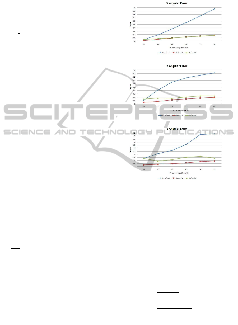
Figure 3: Error results of the synthetic data for all K values:
(d) the average x angular error, (e) the average y angular
error and (f) the average z angular error. Refine1 (red) lines
represent 0% Windprofiler error while Refine2 (green) lines
represent 10% Windprofiler error.
various percentages of Gaussian noise (N[0,1]) to the
synthetic radial velocity data.
2.2 Error Metrics
The quantitative analysis includes the overall output
error, E
O
, and for each voxel, i, the magnitude error,
E
M
i
, the direction error, E
D
i
, and the component an-
gular errors, E
A
x
i
, E
A
y
i
and E
A
z
i
. These error metrics
are defined as:
E
O
=
k
~
V
e
−
~
V
c
k
2
k
~
V
c
k
2
× 100%, (7)
E
M
i
=
|k
~
V
e
i
k
2
− k
~
V
c
i
k
2
|
k
~
V
c
i
k
2
× 100%, (8)
E
D
i
= arccos(
~
V
e
i
·
~
V
c
i
k
~
V
e
i
k
2
k
~
V
c
i
k
2
) ×
180
◦
π
, (9)
3D OPTICAL FLOWFROM DOPPLER AND WINDPROFILER RADAR DATA
677
E
A
x
i
= arccos(
ˆ
V
′
c
x
i
·
ˆ
V
′
e
x
i
), (10)
E
A
y
i
= arccos(
ˆ
V
′
c
y
i
·
ˆ
V
′
e
y
i
), (11)
E
A
z
i
= arccos(
ˆ
V
′
c
z
i
·
ˆ
V
′
e
z
i
), (12)
where
~
V
e
i
is the retrieved velocity at location i and
~
V
c
i
is the correct velocity at location i used by the syn-
thetic data generation. Given estimated velocity
~
V
e
=
(V
e
x
,V
e
y
,V
e
z
) and correct velocity
~
V
c
= (V
c
x
,V
c
y
,V
c
z
),
the component angular error calculation in Equa-
tion (10), for example, uses
~
V
′
e
x
= (V
e
x
,1) and
~
V
′
c
x
=
(V
c
x
,1). Note that we use
ˆ
V to indicate that
~
V has been
normalized. The component angular errors provide a
single numerical value that captures both magnitude
and angular error and avoids the zero division prob-
lem inherent in relative error metrics (Barron et al.,
1994). To summarize the algorithm’s performance as
a whole, we present the averaged metrics below.
3 EXPERIMENTAL RESULTS
Figure 1 shows the unrefined and refined optical flow
for our synthetic data. The blue circle center indi-
cates the position of the Harrow Windprofiler in the
real data (and we use the same position in the syn-
thetic data) while its radius is 2σ
x
(95% confidence).
Note that the velocity in the undefined case is to the
right and downwards while the velocity in the refined
case is also to the right but less downwards. Figs. 2
and 3 shows the various averaged error measures in-
side the Windprofiler 95% confidence circle for the
unrefined (blue) and refined flow for 20% Doppler
data noise and 0% (red) and 10% (green) Windpro-
filer noise. Obviously, the Windprofiler data greatly
improves the flow computation.
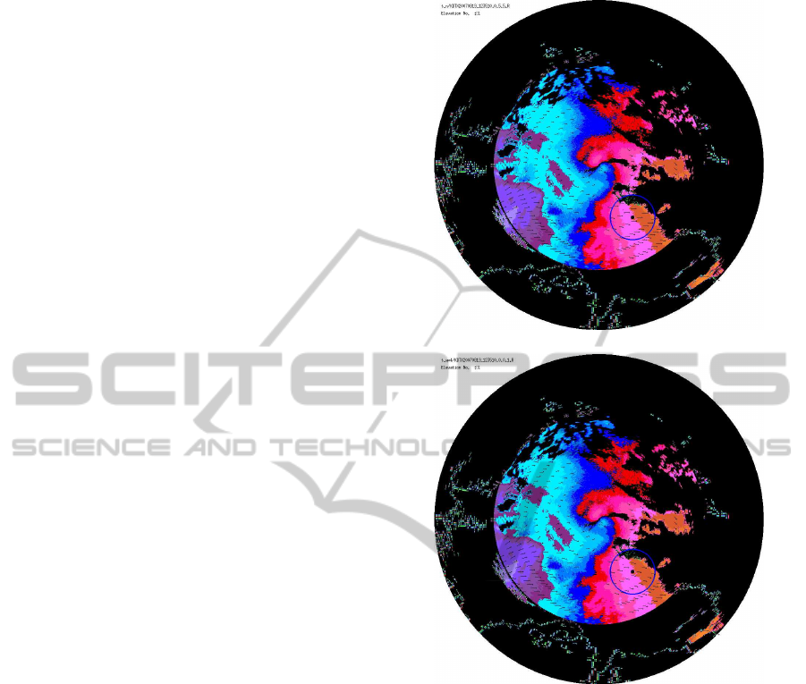
We present some preliminary results for our mea-
sured Doppler and Windprofiler data. Figs. 4a and
4b show the unrefined and refined UV optical flow
fields for the Detroit Doppler data at 12:35:10 of Au-
gust 19
th
, 2007. We also show the W component of
optical flow along the z (height) axis in Figs. 5a and
5b. Component velocities in these figures are shown
as coloured pixels. They correspond to the standard
numerical values used for NEXRADII data. Note that
these component colours have replaced the radial ve-
locity magnitude colours in Figs. 4a and 4b.
It is clear from the z component flow field images
that the refined method significantly changes the flow
field around the Windprofiler radar. Figure 4a has the
unrefined flow going north while Figure 5a has the
refined flow going south. We see a significantly im-
proved recovery of component velocity W in the z di-
rection. In the unrefined component flow shown in
(a)
(b)
Figure 4: Full velocity retrieved from the Detroit Doppler
(and the Harrow Windprofiler) data on August 19
th
, 2007 at
12:35:10: (a) the unrefined UV optical flow and (b) the re-
finedUV optical flow. The blue circle indicates the location
of the Windprofiler radar.
Figure 5a, there is a large area where the component
velocities are the maximum possible value (yellow).
However, in the component flow shown in Figure 5b,
it is obviousthat a more reasonable result has been ob-
tained in the area surrounding the Windprofiler radar.
We observe a strong upward velocity component in
the areas not overlapped by the Windprofiler radar but
a significant downward velocity component in outer
area around the Windprofiler radar. This is due to the
fact that the Windprofiler constraint adopted different
velocity values for the Doppler voxels according to
their actual distances from the Doppler radar points.
VISAPP 2011 - International Conference on Computer Vision Theory and Applications
678

(a)
(b)
Figure 5: Full velocity retrieved from the Detroit Doppler
(and the Harrow Windprofiler) data on August 19
th
, 2007
at 12:35:10: (a) the W component of the unrefined optical
flow and (b) the W component of the refined optical flow.
Again, the blue circle indicates the location of the Wind-
profiler radar.
4 CONCLUSIONS
In this paper we briefly described combining Wind-
profiler data at the Harrow radar station with
NEXRADII Doppler data from Detroit to produce
an arguably more accurate optical flow field in the
vicinity of the Windprofiler radar. We showed that
qualitatively, more accurate and detailed information
could be recovered along the z (height) dimension and
sometimes in the x and y dimensions. However, it is
noted that a Windprofiler radar only covers a small
area compared to a Doppler radar. This limits its ap-
plication. Our framework can handle more Windpro-
filer and Doppler radars but we do not yet have re-
sults for more than one Windprofiler radar data set
and one Doppler radar data set that overlap. We have
recently shown that more accurate optical flow can be
recovered in the overlapping (oval) areas of 2 Doppler
radars (Y. Zhang and Mercer, 2010) using our reg-
ularization framework. Using multiple Doppler and
Windprofiler radars to track storms over long periods
of time is a current area of research.
ACKNOWLEDGEMENTS
We acknowledge funding from the Natural Sciences
and EngineeringResearch Council of Canada, and the
Canadian Foundation for Innovation.
REFERENCES
Barron, J., Fleet, D., and Beauchemin, S. (1994). Perfor-
mance of optical flow techniques. Int. Journal of Com-
puter Vision, 12:43–77.
Barron, J., R.E.Mercer, Chen, X., and Joe, P. (2005). 3d
velocity from 3d doppler radial velocity. Intl. Journal
of Imaging Systems and Technology, 15:189–198.
Easterbrook, C. C. (1975). Estimating horizontal wind
fields by two-dimensional curve fitting of single
doppler radar measurements. In 16th Radar Meteo-
rology Conf., pages 214–219.
Horn, B. K. P. and Schunck, B. G. (1981). Determing opti-
cal flow. Artifical Intelligence, 17:185–204.
Lhermitte, R. M. and Altas, D. (1961). Precipitation motion
by pulse doppler. In 9th Weather Radar Conference,
pages 218–223.
Lucas, B. D. and Kanade, T. (1981). An iterative image-
registration technique with an application to stereo
vision. In DARPA Image Understanding Workshop,
pages 121–130.
Waldteufel, P. and Corbin, H. (1979). On the analysis of
single-doppler radar data. J. of Applied Met., 18:532–
542.
Y. Zhang, J. B. and Mercer, R. E. (2010). 3d optical
flow from single and dual doppler radars. In Irish
Machine Vision and Image Processing Conference
(IMVIP2010).
3D OPTICAL FLOWFROM DOPPLER AND WINDPROFILER RADAR DATA
679
