
OBJECT TRACKING BASED ON PARTICLE FILTERING WITH
MULTIPLE APPEARANCE MODELS
Nicolas Widynski
T
´
el
´
ecom ParisTech, CNRS LTCI, Paris, France
Emanuel Aldea, S
´
everine Dubuisson
University Pierre et Marie Curie, UPMC-LIP6, Paris, France
Isabelle Bloch
T
´
el
´
ecom ParisTech, CNRS LTCI, Paris, France
Keywords:
Object tracking in video Sequences, Particle filter, Multiple appearance models.
Abstract:
In this paper, we propose a novel method to track an object whose appearance is evolving in time. The tracking
procedure is performed by a particle filter algorithm in which all possible appearance models are explicitly
considered using a mixture decomposition of the likelihood. Then, the component weights of this mixture are
conditioned by both the state and the current observation. Moreover, the use of the current observation makes
the estimation process more robust and allows handling complementary features, such as color and shape
information. In the proposed approach, these estimated component weights are computed using a Support
Vector Machine. Tests on a mouth tracking problem show that the multiple appearance model outperforms
classical single appearance likelihood.
1 INTRODUCTION
Using several features or sensors in a tracking particle
filter based procedure has abundantly been studied in
the literature. For instance, the authors in (Brasnett
et al., 2007) propose to combine color, edge and tex-
ture information, (Maggio et al., 2005) use color and
texture, and (Mu
˜
noz-Salinas et al., 2008) use color
and a distance map. Integrating several modalities
into the particle filter is still a challenging problem,
since it requires to take into account the context to
cope with different situations. In (Hotta, 2006; Xu
and Li, 2005), a mixture density is used to model the
likelihood, whose weights correspond to the proba-
bility for the considered modality to be the most rel-
evant one. Confidence exponents in feature likeli-
hoods are considered in (Brasnett et al., 2007; Erdem
et al., 2010), and an uncertainty principle of a fea-
ture with a dispersion criterion of the computed likeli-
hoods in (Maggio et al., 2005). However, most of ex-
isting methods require to evaluate a posteriori the pa-
rameters of the modality relevance, i.e. after the par-
ticle filter estimation, and therefore deliver a unique
set a parameters for the particle cloud. This strategy
may fail, since assigning the same weights to all the
particles may induce error propagations.
In this article, we propose to decompose the like-
lihood into multiple appearance models. This prob-
lem is close to the changing appearance one proposed
in (Nummiaro et al., 2002; Mu
˜
noz-Salinas et al.,
2008). The main difference is that we explicitly
consider several appearance models. This allows us
to use several features in an original way. Further-
more, we consider a mixture likelihood model whose
weights depend on the state and the current observa-
tion, and are then unique for each particle. As an orig-
inal application, we propose to compute the weights
with a Support Vector Machine, and to experiment the
proposed model on a mouth tracking application.
2 PARTICLE FILTERING
Let us consider a classical filtering problem and
denote by x
t
∈ X the hidden state of a stochas-
604
Widynski N., Aldea E., Dubuisson S. and Bloch I..
OBJECT TRACKING BASED ON PARTICLE FILTERING WITH MULTIPLE APPEARANCE MODELS.
DOI: 10.5220/0003334606040609
In Proceedings of the International Conference on Computer Vision Theory and Applications (VISAPP-2011), pages 604-609
ISBN: 978-989-8425-47-8
Copyright
c
2011 SCITEPRESS (Science and Technology Publications, Lda.)

tic process at time t and by y
t
∈ Y the measure-
ment state. The non-linear Bayesian tracking con-
sists in estimating the posterior filtering density func-
tion p(x
t
|y
1:t
) through a non-linear transition function
x
t
= f
t
(x
t−1
, v
t
) and a non-linear measurement func-
tion y
t
= h
t
(x
t
, w
t
). Particle filters, also known as se-
quential Monte-Carlo methods, are used to approxi-
mate the posterior distribution by a weighted sum of
Dirac masses centered on hypothetical state realiza-
tions of the state x
t
, also called particles. For more
details about particle filters techniques, see (Doucet
et al., 2001).
In this paper, we focus on the design of the
likelihood density function induced by h
t
, which is
of prime interest in Bayesian estimation methods,
and especially in a particle filter framework, since
it weights the particle cloud. As we will see in the
next section, using several features or sensors usually
helps, but imposes to properly model these different
pieces of information, which can be redundant or con-
flicting. In Section 4, we propose a new method for
integrating several features in the likelihood process,
by partitioning the space of the object feature, leading
to a mixture of likelihood density functions.
3 STATE OF THE ART
Using several features, several sensors, or several ap-
pearance models, are distinct concepts. In the parti-
cle filter framework, multi-sensors models and multi-
features ones often lead to similar implementations,
and are therefore not always clearly distinguished in
the literature. Here we use the term multi-modalities
to denote these two types of data. We describe next
two popular models, which are suited in most cases,
dealing with several features of several sensors.
In the following, x
t
∈ X denotes the hidden state
of a stochastic process at time t, and y
t
= (y
1
t
, . . . , y
R
t
)
is a vector of R components, where y
r
t
stands for the
r
th
modality.
The first model consists in factorizing the like-
lihood density as a mixture model, in which
each component represents a modality: p(y
t
|x
t
) =
∑
R
r=1
π
r
t
p(y
r
t
|x
t
), with {π
r
t
}
R
r=1
the “relevance proba-
bility” of the modalities (
∑
R
r=1
π
r
t
= 1), i.e. the prob-
ability that the modality r is the one which describes
the state x
t
. These probabilities are either fixed by
hand (Xu and Li, 2005), or adaptive but with a fixed
set a possible values (Hotta, 2006).
The second model introduces confidence or reli-
abilitiy in a modality. It considers a conditional in-
dependence between the modalities according to the
state x
t
. Confidence indices {α
r
t
}
R
r=1
are then added in
a ad hoc way as exponents of the marginal likelihoods
p(y
r
t
|x
t
), r = 1, . . . , R: p(y
t
|x
t
) =
∏
R
r=1
p(y
r
t
|x
t
)
α
r
t
,
with α
r
t
∈ [0, 1]. The values α
r
t
represent the confi-
dence in the modality r. Unlike the first model, in-
dices α
r
t
are independent of each other, which facili-
tates their update. They can be defined using differ-
ent features, one can see for example (Brasnett et al.,
2007; Erdem et al., 2010).
When the appearance of the object evolves dur-
ing time, for example because of luminosity or pose
changes, tracking algorithms using a correlation cri-
terion between a reference model and a candidate
must update the reference model to stay robust. The
implementation of a model with a changing appear-
ance consists in updating progressively the reference
model, as it has notably been proposed in (Nummiaro
et al., 2002; Mu
˜
noz-Salinas et al., 2008).
Here, instead of updating the reference model, we
propose a different approach, that explicitly models
several components which may be related to several
appearances.
All methods described in this section aim at defin-
ing adaptive weights, of probability, confidence or
model update. This adaptive feature enhances the
models with more flexibility and robustness. How-
ever, the update is often difficult and therefore often
performed in an heuristic way, by computing the val-
ues a posteriori according to a defined criterion. The
strategy is therefore not directly included in the par-
ticle filter framework, and delivers a single parameter
set for all the particles. Hence, errors can propagate
and accumulate during time, thus definitely biasing or
deteriorating the reference model. This may lead to
unsuitable likelihoods and penalize the tracking task.
The model we propose defines the likelihood by a
mixture of densities, in which each particle is associ-
ated with a different set of weights. Hence, this strat-
egy does not suffer from the aforementioned problem.
The originality comes from the fact that a weight is
related to a decomposition of the state and the obser-
vation and not to a feature or a sensor.
4 MULTIPLE MODEL
LIKELIHOOD
We propose in this section to define a multiple model
likelihood. We consider that an appearance is a possi-
ble representation of an object, according to a con-
sidered feature. This modeling is useful when ob-
ject appearance (color, shape,...) changes during time.
For example, in a 3D face tracking problem, one may
define several components, that we call postures, for
which the probabilities are computed using the ori-
OBJECT TRACKING BASED ON PARTICLE FILTERING WITH MULTIPLE APPEARANCE MODELS
605

entation of the head (front, profile and behind), and
associated with a color likelihood, conditioned by the
considered posture. The appearance corresponds to
the reference model used by the color likelihood. In
this case, the orientation criterion defines the type of
posture that the object describes. By defining the joint
likelihood by a mixture density, component weights
are defined using the orientation of the head, and al-
lows integrating in an original way complementary
features in the joint likelihood density.
We describe now the formalization of the pro-
posed approach. Let
•
x = (
•
x
1
, . . . ,
•
x
O
) be a vector
of O components, where
•
x
j
represents the reference
model (the appearance) of the object, associated with
the component j denoting a posture. For example, if
j = 2 represents the posture behind a face (this com-
ponent being defined from some information on the
orientation of the head), a color based on appearance
model
•
x
2
will be described by the color of the hair.
The joint likelihood is given by:
p(y
t
|x
t
,
•
x) =
O
∑
j=1
ϕ
j
(γ(x
t
, y
t
)) p(y
t
|x
t
,
•
x
j
) (1)
with p(y
t
|x
t
,
•
x
j
) the likelihood of the component j
and ϕ
j
(γ(x
t
, y
t
)) the weight of the posture j associ-
ated with the feature γ(x
t
, y
t
), with ϕ
j
: Z → [0, 1]
such that ∀(x
t
, y
t
) ∈ X × Y,
∑
O
i=1
ϕ
i
(γ(x
t
, y
t
)) = 1,
with Z the feature space, and γ : X × Y → Z the fea-
ture function. Index j represents the j
th
posture of
the decomposition, and ϕ
j
(γ(x
t
, y
t
)) the probability
of the posture j.
Observations considered for the weights and the
likelihoods may be of different kinds. For example,
in a 3D face tracking application, the posture proba-
bilities, based on the orientation of the head, may be
computed using gradient information extracted from
the input image, whereas likelihoods conditioned by
the appearance models may be defined by a distance
between color histograms. Observations are respec-
tively noted y
App
t
and y
Pos
t
. Equation 1 becomes:
p(y
t
|x
t
,
•
x) '
O
∑
j=1
ϕ
j
γ(x
t
, y
Pos
t
)
p(y
App
t
|x
t
,
•
x
j
) (2)
This equation is obtained by considering the condi-
tional independence of the weights with respect to
y
App
t
given y
Pos
t
, and the term p(y
Pos
t
|x
t
,
•
x
j
, y
App
t
) is
simply ignored, since this approximation allows us to
make the desired distinction between “posture” and
“appearance” information, and does not necessarily
require the existence of y
Pos
t
. An original feature of
this decomposition is the conditioning of the weights
with respect to x
t
and y
Pos
t
. This means they are auto-
matically determined by the current observation, and
dedicated to the considered particle, which contrasts
with existing methods (see Section 3).
Although the application field seems to be vast,
we choose to define the weights ϕ
j
γ(x
t
, y
Pos
t
)
as to
be dependent of the state x
t
and the observation y
t
, in
order to show the modeling potential of the approach.
Furthermore, although these weights might be, in
many applications, defined by a known closed-form γ,
we are interested in the case where they are learned.
When the learning database is not labeled, a clustering
technique such as k-means algorithm (Dhillon et al.,
2004) or an unsupervised classifier (Ben-Hur et al.,
2002) can be employed. In this work, we consider
a labeled learning database, where the labels are the
indices characterizing the postures and are assumed
to be known. The methodology consists in using a
supervised classifier, here a Support Vector Machine
(SVM), in the feature space Z, which allows comput-
ing the probability of a couple (x
t
, y
Pos
t
) to belong to
a class j thanks to the feature function γ. The choice
of a SVM is motivated by its efficiency, its generic-
ity, and its capability to provide a classification result
in the form of probabilities, which will then be inte-
grated in the likelihood model.
5 LEARNING USING SUPPORT
VECTOR MACHINES
In the proposed model, the considered classes
are the postures, and a SVM classifier is used to
automatically determine membership weights to
classes. Considering a SVM output interpreted as
posterior probabilities (Platt, 2000), we use a strategy
of pairwise coupling to compute the probabilities
p
j
= Pr(l = j|z), j = 1, . . . , O (Wu et al., 2004),
with O the number of classes, here the number of
postures. In the model proposed in Equation 2, the
value p
j
corresponds to the probability to consider
the j
th
posture of the model, i.e. ϕ
j
γ(x
t
, y
Pos
t
)
.
We consider
O
2
SVM with a learning database D =
n
γ(x
(1)
, y
Pos,(1)
), l
(1)
, . . . ,
γ(x
(M)
, y
Pos,(M)
), l
(M)
o
,
with γ the feature function, and l
(M)
the la-
bel, which denotes the posture index, and
so implicitly the appearance. The weights
ϕ
j
γ(x
t
, y
Pos
t
)
are then given by probabilities
{p
j
}
O
j=1
: ∀ j ∈ {1, . . . , O}, ϕ
j
γ(x
t
, y
Pos
t
)
= Pr(l =
j|γ(x
t
, y
Pos
t
)) = p
j
.
We can also use the membership probabilities
of samples from the learning database to build ap-
pearance models {
•
x
j
}
O
j=1
. They are defined as the
weighted sum of the samples where the weights are
VISAPP 2011 - International Conference on Computer Vision Theory and Applications
606

the membership probabilities to the considered class:
•
x
j
=
∑
M
i=1
Pr
l = j|γ(x
(i)
, y
Pos,(i)
)
η(x
(i)
)
∑
M
i=1
Pr
l = j|γ(x
(i)
, y
Pos,(i)
)
(3)
where Pr
l = j|γ(x
(i)
, y
Pos,(i)
)
is the probability
to consider the posture j according to the data
γ(x
(i)
, y
Pos,(i)
), extracted from a pairwise coupling
strategy, and η is a function characterizing an appear-
ance, which will be formalized in Section 6.
6 EXPERIMENTS
We consider an application of mouth tracking, us-
ing one, two and three postures. The purpose of
these experiments is to show the interest of using
several postures into a general particle filter frame-
work, and not to compare results to the ones obtained
by mouth tracking dedicated methods. Likelihoods
{p(y
t
|x
t
,
•
x
j
)}
O
j=1
are based on color information, and
use the reference histograms {
•
x
j
}
O
j=1
. Experiments
will use different posture weights: color histogram
features with a Bhattacharyya distance, or shape fea-
tures with an Euclidean or a Hausdorff distance.
We propose to use the learning and test sets
coming from an annotated database freely available
on the Internet
1
. This sequence contains 5000 im-
ages showing a human face with changing expres-
sions (Figure 1). The learning database contains
1000 elements. Each of these elements is a mouth
shape defined by a set of P control points, from
which we extract a color histogram. Let D =
n
γ(z
(1)
), l
(1)
, . . . ,
γ(z
(M)
), l
(M)
o
be M samples
of the learning database, with γ(z
(i)
) the feature func-
tion used in the SVM extracted from the i
th
shape z
(i)
.
We propose to track the mouth in a 300 image se-
quence (not used for the learning database contruc-
tion). For comparison, we consider three decomposi-
tions of the joint likelihood: a decomposition in one
element, mouth, which corresponds to a classical case
(i.e., no classification); a decomposition in two ele-
ments, closed mouth and open mouth (which includes
elements open mouth and smile); and finally a decom-
position in three elements, closed mouth, open mouth,
and smile.
The state vector x
t
= (x
t
, y
t
,
˙
x
t
,
˙
y
t
, θ
t
, a
t
) contains
the 2D coordinates (x
t
, y
t
) of the center of the mouth
at time t, the velocity (
˙
x
t
,
˙
y
t
), the orientation of the
1
http://personalpages.manchester.ac.uk/staff/
timothy.f.cootes/data/talking face/talking face.html
(a) (b) (c)
Figure 1: Images taken from the tested sequence, showing
samples of three classes of posture for the mouth (a) closed
mouth, (b) open mouth and (c) smile.
mouth θ
t
and a set of control points a
t
= (a
1
t
, . . . , a
P
t
).
We consider a constant velocity model. The dynam-
ical model for the parameters (
˙
x
t
,
˙
y
t
, θ
t
, a
t
) is the one
proposed in (Widynski et al., 2010), which specifi-
cally allows us to, in particular, handle non rigid shape
transformations.
We consider a likelihood p(y
App
t
|x
t
,
•
x
j
) combin-
ing color and edge information: p(y
App
t
|x
t
,
•
x
j
) =
p(y
App,R
t
|x
t
,
•
x
j
) p(y
App,C
t
|x
t
), where p(y
App,C
t
|x
t
) is
an edge likelihood based on gradient values com-
puted on the B-Spline interpolation of the con-
trol points a
t
at position (x
t
, y
t
) and orientation θ
t
,
and p(y
App,R
t
|x
t
,
•
x
j
) a region likelihood, conditioned
by the j
th
reference model. The region likeli-
hood uses a notion of distance between HSV his-
tograms (P
´
erez et al., 2002). Both likelihoods are also
explained in (Widynski et al., 2010). Reference his-
tograms {
•
x
j
}
O
j=1
are computed automatically using
the SVM (Equation 3), with γ(x
(i)
, y
Pos,(i)
) = γ(z
(i)
)
and η(x
(i)
) = h(z
(i)
), where γ(z
(i)
) is the feature func-
tion, and h(z
(i)
) the histogram extracted from the sam-
ple z
(i)
of the learning database. The joint likelihood
considering O components for the color likelihood is
finally written by:
p(y
t
|x
t
,
•
x) =
h
O
∑
j=1
ϕ
j
γ(x
t
, y
Pos
t
)
p(y
App,R
t
|x
t
,
•
x
j
)
i
× p(y
App,C
t
|x
t
) (4)
It only remains to define the function γ in order to
construct the SVM classifier.
We consider Gaussian kernels, in order to obtain
a non linear separation of the data, K(γ(z
(i)
), γ(z)) =
exp
−
hγ(z
(i)
),γ(z)i
2
2σ
2
, with z
(i)
the i
th
shape of mouth
from the learning database, z a candidate shape of
mouth (or while learning, a shape z
(i)
from the
database), σ
2
the fixed variance, and h.i the norm that
depends on the type of feature used.
As a first criterion characterizing a component
probability of the model, we consider color his-
tograms. The feature function γ corresponds to a
region histogram, hence γ(x
t
, y
Pos
t
) = h( ˚a
t
), with ˚a
t
the set of points belonging to the region described by
(x
t
, y
t
, θ
t
, a
t
). The kernel norm of the SVM is a Bhat-
OBJECT TRACKING BASED ON PARTICLE FILTERING WITH MULTIPLE APPEARANCE MODELS
607

tacharyya distance.
As a second experiment, we use a shape infor-
mation to compute component probabilities. In this
case, the weight function of the posture does not de-
pend on the observation, since we only consider a
set of 2D points. Hence γ is written by the set of
control points a
t
, and ϕ
j
γ(x
t
, y
Pos
t
)
= ϕ
j
(γ(x
t
)) =
ϕ
j
(γ(z)) = ϕ
j
(a
t
). The Euclidean norm is used to
compute the distance between two shapes.
For the last experiment, we use a Hausdorff dis-
tance criterion. Like for the Euclidean distance, the
weight function does not depend on the observation,
and the weights are ϕ
j
γ(x
t
, y
Pos
t
)
= ϕ
j
(a
t
).
Mean tracking errors over 300 images with the
three proposed experiments are given in Figure 2, ac-
cording to the number of particles. Error at time t
corresponds to 1 minus the ratio between common
points of the estimated shape and the true shape and
the largest area of these two objects. The benefice of a
multi-appearance model is clear, since, for all criteria,
the decreasing error between one and two postures is
nearly equals to 25%. Between two and three pos-
tures, the difference is less important, since the parti-
tioning is less obvious than with two postures.
Comparisons between criteria are given in Fig-
ure 3. We can see that the histogram criterion gives
better results than the shape criteria, probably thanks
to the quantity of information contained in such a
model, which gives a robust weight estimation, even
for noisy environments.
Figure 4 illustrates image results with one, two
and three classes. The estimated mouth is in blue and
corresponds to the Monte-Carlo expected value. The
used criterion is the color histogram distance since,
as we saw, it provides the best results. The difference
between the results obtained with one and two/three
postures is clear, as we can see on images 2 to 4. Be-
tween two and three postures, estimations on images
2 to 4 also present differences, even if they are less ob-
vious. In particular, the orientation of the mouth esti-
mated in the fourth image with two postures is clearly
less better than with three.
Since we consider a multiple model likelihood, the
number of decomposition O directly affects the com-
putational time of the proposed approach, since the
method requires to compute the likelihood densities
{p(y
App
t
|x
t
,
•
x
j
)}
O
j=1
. Moreover, the overall computa-
tional time also depends on the computation of the
weights ϕ
j
. In our experiments, the weights are es-
timated using the output of SVM, and then only re-
quires to compute distances of the data to the sup-
port vectors, which is fast while the number of sup-
port vectors and the computational time of the dis-
tance stay reasonable.
Error
Number of particles
1 posture
2 postures
3 postures
(a)
Error
Number of particles
1 posture
2 postures
3 postures
(b)
Error
Number of particles
1 posture
2 postures
3 postures
(c)
Figure 2: Mouth tracking errors obtained using as weight-
ing criteria an information of (a) shape with an Euclidean
distance, (b) shape with a Hausdorff distance, and (c) color
with a Bhattacharyya distance.
Error
Number of particles
Color histogram dist.
Shape dist. Euclidean
Shape dist. Hausdorff
(a)
Error
Number of particles
Color histogram dist.
Shape dist. Euclidean
Shape dist. Hausdorff
(b)
Figure 3: Mouth tracking errors obtained using different
criteria to weight the likelihoods, with (a) two postures, and
(b) with three postures.
7 CONCLUSIONS
We proposed in this article a multiple model likeli-
hood. The originality of this work is twofold: first,
each model is related to an object appearance, an ap-
proach that has never been employed. Secondly, the
model implementation uses a decomposition of the
VISAPP 2011 - International Conference on Computer Vision Theory and Applications
608
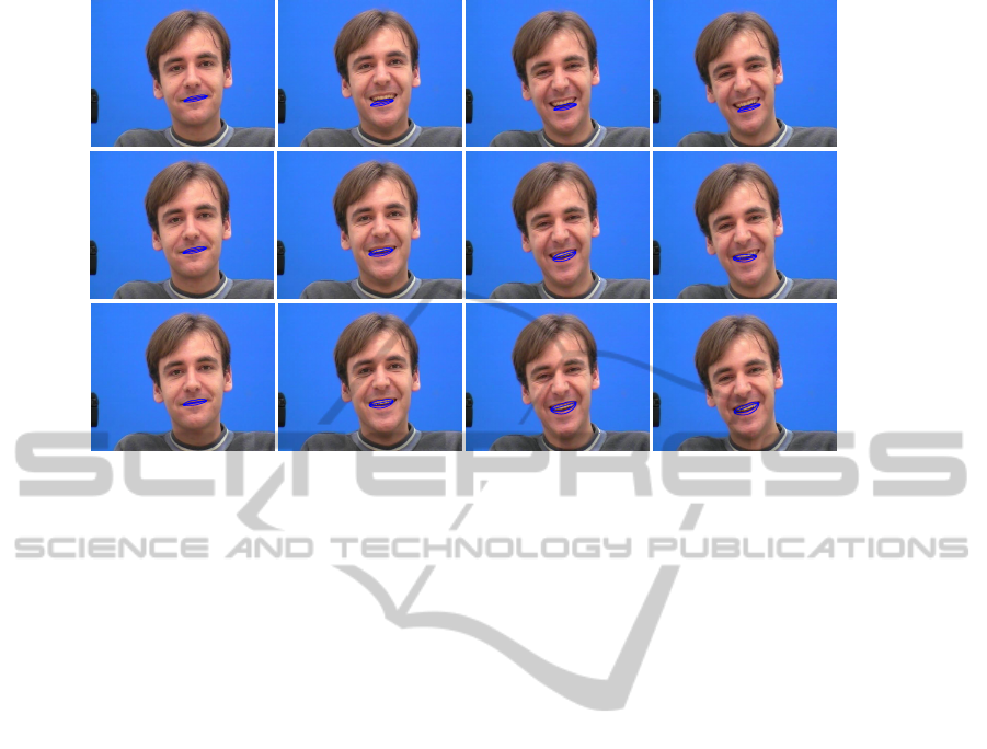
(a)
(b)
(c)
Figure 4: Captions of results obtained with (a) one, (b) two, and (c) three postures, in a test sequence of 300 images. The
estimated shape is illustrated in blue.
likelihood as a mixture model, whose weights are de-
termined according to the state and the observation
at time t, so weights are unique by particle. This
problem, which is a part of our contribution, allows
dealing with many applications, improving the track-
ing robustness while using in an original way several
modalities. To compute the weights, we proposed
to use a SVM, that separates offline the considered
features. We tested our method on a mouth track-
ing problem. Experiments have shown that using few
components, i.e. few postures, improves significantly
the results, since while refining the description model
it robustifies the likelihood.
REFERENCES
Ben-Hur, A., Horn, D., Siegelmann, H., and Vapnik, V.
(2002). Support vector clustering. The Journal of Ma-
chine Learning Research, 2:125–137.
Brasnett, P., Mihaylova, L., Bull, D., and Canagarajah, N.
(2007). Sequential Monte Carlo tracking by fusing
multiple cues in video sequences. Image Vision Com-
puting, 25(8):1217–1227.
Dhillon, I., Guan, Y., and Kulis, B. (2004). Kernel k-
means: spectral clustering and normalized cuts. In
ACM SIGKDD, pages 551–556.
Doucet, A., De Freitas, N., and Gordon, N., editors
(2001). Sequential Monte Carlo methods in practice.
Springer.
Erdem, E., Dubuisson, S., and Bloch, I. (2010). Particle
Filter-Based Visual Tracking by Fusing Multiple Cues
with Context-Sensitive Reliabilities. Technical Report
2010D002, T
´
el
´
ecom ParisTech.
Hotta, K. (2006). Adaptive Weighting of Local Classifiers
by Particle Filter. In ICPR, volume 2, pages 610–613.
Maggio, E., Smeraldi, F., and Cavallaro, A. (2005). Com-
bining colour and orientation for adaptive particle
filter-based tracking. In British Machine Vision Con-
ference, pages 659–668.
Mu
˜
noz-Salinas, R., Aguirre, E., Garc
´
ıa-Silvente, M., and
Gonzalez, A. (2008). A multiple object tracking ap-
proach that combines colour and depth information
using a confidence measure. Pattern Recognition Let-
ters, 29(10):1504–1514.
Nummiaro, K., Koller-Meier, E., and Gool, L. V. (2002).
Object Tracking with an Adaptive Color-Based Parti-
cle Filter. In Symposium for Pattern Recognition of
the DAGM, pages 353–360.
P
´
erez, P., Hue, C., Vermaak, J., and Gangnet, M. (2002).
Color-Based Probabilistic Tracking. In ECCV, pages
661–675.
Platt, J. C. (2000). Probabilistic Outputs for Support Vec-
tor Machines and Comparisons to Regularized Likeli-
hood Methods. In Advances in Large Margin Classi-
fiers, pages 61–74.
Widynski, N., Dubuisson, S., and Bloch, I. (2010). Integra-
tion of fuzzy spatial information in tracking based on
particle filtering. IEEE Transactions on Systems, Man
and Cybernetics SMCB, To Appear.
Wu, T.-F., Lin, C.-J., and Weng, R. C. (2004). Probabil-
ity estimates for multi-class classification by pairwise
coupling. Journal of Machine Learning Research,
5:975–1005.
Xu, X. and Li, B. (2005). Rao-Blackwellised particle filter
for tracking with application in visual surveillance. In
IEEE International Workshop on Visual Surveillance
and Performance Evaluation of Tracking and Surveil-
lance, pages 17–24.
OBJECT TRACKING BASED ON PARTICLE FILTERING WITH MULTIPLE APPEARANCE MODELS
609
