
TEMPORAL BAG-OF-WORDS
A Generative Model for Visual Place Recognition using Temporal Integration
Herv
´
e Guillaume
∗†
, Mathieu Dubois
∗†
, Emmanuelle Frenoux
†∗
and Philippe Tarroux
†‡
∗
Univ Paris-Sud, Orsay, F-91405, France
†
LIMSI - CNRS, B.P. 133, Orsay, F-91403, France
‡
Ecole Normale Suprieure, 45 rue d’Ulm, Paris, F-75230, France
Keywords:
Place recognition, Bag-of-Words, Temporal integration, Generative learning.
Abstract:
This paper presents an original approach for visual place recognition and categorization. The simple idea
behind our model is that, for a mobile robot, use of the previous frames, and not only the one, can ease
recognition. We present an algorithm for integrating the answers from different images.
In this perspective, scenes are encoded thanks to a global signature (the context of a scene) and then classified
in an unsupervised way with a Self-Organizing Map. The prototypes form a visual dictionary which can
roughly describe the environment. A place can then be learnt and represented through the frequency of the
prototypes. This approach is a variant of Bag-of-Words approaches used in the domain of scene classification
with the major difference that the different “words” are not taken from the same image but from temporally
ordered images. Temporal integration allows us to use Bag-of-Words together with a global characterization
of scenes. We evaluate our system with the COLD database. We perform a place recognition task and a place
categorization task. Despite its simplicity, thanks to temporal integration of visual cues, our system achieves
state-of-the-art performances.
1 INTRODUCTION
Mobile robot localization has been an intensive field
of study in the past decades (see (Filliat and Meyer,
2003)). Traditional approaches have focused on met-
ric localization (i.e. the ability to position objects in a
common coordinate frame) or topological localization
(i.e. the ability to build a graph of interesting places).
However in those approaches, a place does not neces-
sary coincide with the human concept of rooms. In
this paper the word “place” designates a particular
room such as office 205, the corridor of the second
floor, etc. Recently research had focused on seman-
tic place recognition which is the ability for a mo-
bile robot to recognize the room (kitchen office) it is
currently in and the nature of its environment. The
knowledge of the semantic context allows to draw hy-
pothesis on the identity of perceived objects (see (Tor-
ralba, 2003)). There is a huge semantic gap between
the human notion of room and sensor measurements
available to the robot. Therefore, contrary to SLAM
or topological mapping, semantic place recognition is
a supervised problem.
Several solutions have been proposed for place
recognition and place categorization using vision
alone or combined with several types of telemeters
(laser, sonar) (see (Pronobis et al., 2010)). Vision pro-
vides richer information than telemeters which is an
essential advantage for fine discrimination and cat-
egorization of places according to semantic criteria.
That's why vision receives an increasing attention in
the community of place recognition.
Nevertheless, visual recognition and moreover vi-
sual categorization of places is still an open problem
due to at least three major problems. First, the size of
the input space is large due to the size of images. Sec-
ond, the inter-class distance is small (different classes
share common visual features) while the intra-class
distance is large (for instance, an office in a laboratory
can look very different from an office in another labo-
ratory). Last but not least, applications on a real robot
enforce on-line and real-time algorithms (potentially
with low computational resources).
Most works tackle the problem of visual place
recognition as a problem of scene classification i.e.
each frame taken by the robot is assigned to a place.
We think that place recognition is a slightly differ-
ent problem as a single frame may be intrinsically
286
Guillaume H., Dubois M., Frenoux E. and Tarroux P..
TEMPORAL BAG-OF-WORDS - A Generative Model for Visual Place Recognition using Temporal Integration.
DOI: 10.5220/0003353202860295
In Proceedings of the International Conference on Computer Vision Theory and Applications (VISAPP-2011), pages 286-295
ISBN: 978-989-8425-47-8
Copyright
c
2011 SCITEPRESS (Science and Technology Publications, Lda.)

ambiguous, non-informative or even misleading for
place recognition. Imagine that the robot is in an of-
fice but faces a window. The scene will contain trees,
cars, other buildings, etc. A scene classification algo-
rithm might assign the label “outside” to the image.
This example illustrates very well the difference be-
tween scene classification (which basically answers
the question “What am I seeing right now?”) and
place recognition (which answers the question “Ac-
cording to what I am seeing, in which place am I?”).
This article presents two contributions. First,
we develop a method which takes advantage the ex-
ploratory capacity of a robot. The main idea is to
collect several cues during the exploration to disam-
biguate the current scene. While a scene can be am-
biguous a collection of scenes is generally not: for in-
stance in the case of a robot facing a window at time
t, the robot might at time t + 1 face a stair indicating
that it is in the entrance of the laboratory.
Second, we present a system for place recogni-
tion which illustrates this idea. Our system can be
briefly described as follows. Each scene is charac-
terized thanks to a coarse global vector (the visual
context) and each vector is quantized with a vector
quantization algorithm. Thus, we obtain a visual dic-
tionary (or codebook) which allow us to describe the
environment in terms of visual words (i.e. visual scene
prototypes). During the learning stage, each place is
described by the respective frequencies of the proto-
types. Finally, during the recognition phase, the clas-
sification output is obtained thanks to the last L obser-
vations done during exploration. Our method can be
seen as a modification of the Bag-of-Words algorithm
(see (Csurka et al., 2004)) with two major differences:
1. The different words are not taken from the same
image but from temporally ordered images 2. Tempo-
ral integration allows us to use Bag-of-Words together
with a global characterization of scenes.
The rest of the paper is organized as follows. Sec-
tion 2 presents related work. Section 3 presents the
descriptor used and the constitution of the visual dic-
tionary. Section 4 presents the place models and the
Bayesian formalism used for cue integration. Sec-
tion 5 shows the results of our system in a place recog-
nition task and section 6 in a place categorization task.
2 RELATED WORKS
The vast majority of works on place recognition use
techniques developed for scene classification. Some
of them rely on prior object identification (see for
instance (Vasudevan and Siegwart, 2008)). How-
ever most of the recent scene classification and place
recognition systems bypass this step due to its high
complexity and because high performances can be
reached without it.
In this case, the authors usually compute var-
ious descriptors on laser range scans (see for in-
stance (Mozos et al., 2005; Mozos, 2008)) or on
images (using either perspective or omnidirectional
cameras). Multi-modal approaches also exist (see
for instance (Pronobis et al., 2010)). Among vision-
based methods we can distinguish between methods
using global images features (see (Walker and Malik,
2004; Oliva and Torralba, 2001; Pronobis et al., 2006;
Orabona et al., 2007; Torralba et al., 2003)) and meth-
ods using local descriptors (Ullah et al., 2008; Filliat,
2008; Ni et al., 2009) usually computed around inter-
est points. Colours and orientations are the most used
features.
One such local method is the Bag-of-Words model
(BoW) (see (Gokalp and Aksoy, 2007; Fei-Fei and
Perona, 2005; Lazebnik et al., 2006)). The main
idea is to define a visual dictionary by mean of a
vector quantization algorithm. The major advantage
is that quantization decreases the computational cost
of learning while keeping a good classification rate.
BoW has been used in the domain of semantic place
recognition (see (Filliat, 2008) for instance).
In (Pronobis and Caputo, 2007) the authors use a
confidence criterion to compute several cues from the
same image. The idea is first to compute a simple cue
to classify the image. If the confidence is not high
enough then compute another cue and combine those
decisions. This process is repeated until confidence
is sufficiently high (or no more cues are available).
Again, contrary to the work presented here, recogni-
tion is carried out using only one image.
In (Pronobis et al., 2010), the authors use a sim-
ple spatio-temporal accumulation process to filter the
decision of a discriminative confidence-based place
recognition system (which uses only one image to
recognize the place). The responses of the system
are accumulated spatially and temporally along the
robot’s trajectory, thanks to odometric information,
creating a sparse 3D-histogram. The answer of the
system is then the average over space of the accu-
mulated responses. The size of the bins must be ad-
justed so that each bin roughly corresponds to a sin-
gle viewpoint. One problem with this method is that
the system needs to wait some time before giving a
response. Also special care must be taken to detect
places boundaries.
Some authors (Mozos, 2008; Torralba et al., 2003)
use the topology of the environment to predict the
transition between two places and increase general
performance. These works use a Hidden Markov
TEMPORAL BAG-OF-WORDS - A Generative Model for Visual Place Recognition using Temporal Integration
287

Model (HMM) where each place is a hidden state of
the HMM and the feature vector stands for the ob-
servations. One drawback, as there is no quantiza-
tion, is that the input space is continuous and high-
dimensional. The learning procedure is then compu-
tationally expensive.
The work that is the closest to our is (Wu et al.,
2009). The author proposed a system based on quan-
tized descriptors (i.e. a BoW model) in conjunction
with Bayesian Filtering. Our method can be seen as
a simplification of this method since we don’t need to
learn or make assumptions on the probabilities of the
transition between places.
Compared to the previous works, one original-
ity of our system is to combine BoW modelling and
global features instead of local ones. This is made
possible because visual cues are collected over time
instead of being collected over the current visual
scene.
3 OVERVIEW OF THE SYSTEM
Our system is an adaptation of the classic BoW sys-
tem. Each image is described by a global signature
(i.e. a numerical feature vector): at each time step t,
the input image I(t) is presented to the system and its
signature is computed. There are two learning phases.
The first step is to train a vector quantization al-
gorithm. Once this is done, an image can be mapped
to a predetermined vector (i.e. a prototype). One im-
age is then represented by an integer o(t) = k ∈
{
1..S
}
which identifies the prototype (S is the number of pro-
totypes). The set of prototypes is the vocabulary that
will be used for learning places.
Then learning of the place model can take place.
Training is supervised so each observation is labelled
with the name of the place c
i
∈ C we are currently
in (C denotes the set of places in the current environ-
ment).
3.1 Image Signatures
To characterize the images we use two recent global
descriptors that have been developed in the context
of place recognition: GIST (see (Oliva and Torralba,
2001)) and CENTRIST (see (Wu et al., 2009)). Those
descriptors are global i.e. they use all the pixels to
compute the signature (there is no extraction of inter-
est points). Thus we say that they capture the visual
context of the image.
GIST has been proposed in (Oliva and Torralba,
2001) as a global holistic representation of a scene.
It was successfully used for outdoor scene classifica-
tion. GIST is based on the output of a Gabor-like filter
bank (we use 4 scales and 6 orientations) applied on
each colour channel. The 4 × 6 × 3 = 72 resulting
images are evenly divided into 4 × 4 sub-windows.
The output of the filter is averaged on each sub-
window and the resulting vectors are concatenated.
We used the C implementation proposed in (Douze
et al., 2009). To further reduce the dimensionality we
project the 4×4×72 = 1152-dimensional vector onto
the 80 first principal components (which explain more
than 99% of the variance) computed on a database
made of
1
2
images in the COLD database. The sig-
nature captures the most significant spatial structure
in the image.
CENsus TRansform hISTogram (CENTRIST)
was proposed by (Wu et al., 2009) for a place cate-
gorization task. First, the edges of the image are com-
puted using a first-order Sobel filter. The image is
then transformed using Census Transform (CT). This
transformation is similar to LBP
8,1
(see (Ojala et al.,
2002)) and captures the local intensity pattern of the
edges. This transformation is robust to illumination
and gamma changes. The CENTRIST descriptor is
the 256-bins histogram of the CT values. Note that
contrary to (Wu et al., 2009) we do not divide the im-
age in sub-windows. Instead we use only one his-
togram for all the pixels in the image.
3.2 The Self-organizing Map and its
Training
The vector quantization algorithm chosen in this pa-
per is the Self-Organizing Map (SOM) (Kohonen,
1990). It consists in a neural network where neurons
are disposed on a lattice. In this article we will inves-
tigate square maps of different sizes S (ranging from
5 ×5 to 20×20) with a toroidal topology and a Gaus-
sian neighbourhood. Each neuron (or unit) holds a
weight vector (of the same size than the signature).
The SOM needs to be trained with the input vec-
tors (this step should not be confused with the super-
vised learning of the places’ models). At the end of
the learning phase the SOM describes a discrete ap-
proximation of the distribution of training samples.
This process has been shown to form clusters of sim-
ilar images (see (Guillaume et al., 2005)). In the fol-
lowing of this article we shall call “visual prototypes”
or “syntactic categories” the SOM’s neurons. The
set of all the prototypes form a dictionary of visual
scenes.
In the current set-up the training of the SOM is
performed off-line. The off-line training is supposed
to give innate syntactic categories. That’s why we
VISAPP 2011 - International Conference on Computer Vision Theory and Applications
288

have trained the SOMs with a representative sample
of the visual environment made of
1
3
the images of
the COLD database (see section 5).
3.3 Place Models
Once the training of the SOM done we can start to
learn the place models. Because the vocabulary is
discrete and finite we can use a non-parametric ap-
proach. We have chosen to use Naive Bayes Classifier
(NBC). Despite being a very simple generative model
the NBC is able to compete with most discriminative
algorithms (see (Ng and Jordan, 2002)).
We learn one classifier per place. The model of
a place is simply the distribution of the visual proto-
types found during learning which approximates the
likelihood P(o(t)|c
i
). To avoid null values due to
small training set we use the Laplace estimator.
Another interesting feature of our algorithm is that
it is incremental and on-line (once the training of the
SOM is done) and has a low computational complex-
ity due to the discretization of the input space. The
advantage over the work presented in (Mozos, 2008;
Torralba et al., 2003) is that there are no hidden states.
In our case the mapping of an image to a prototype
gives its syntactic category.
4 FRAMEWORK FOR CUE
INTEGRATION
We present here the framework for the temporal inte-
gration of cues which is the main contribution of this
paper. This framework is also based on the Bayes for-
mula but this should not be confused with the NBC
learning and training. As discussed in previous sec-
tions it is interesting for the robot to combine the in-
formations from different images to take advantage
of the spatial extension of a place and its ability to
explore it.
During learning, each image is processed sepa-
rately. During recognition the robot will gather a set
of observations with a sliding window of size L:
O
L
(t) =
{
o(t − L + 1), . . . , o(t − 1), o(t)
}
We seek for the place c
∗
which maximizes the a
posteriori probability for a given sequence O
L
(t):
c
∗
= argmax
c
i
∈C
P(c
i
|O
L
(t)) (1)
If we consider that the L observations are indepen-
dent and using Bayes' rule we have:
c
∗
= argmax
c
i
∈C
t
∏
t
0
=t−L+1
P(c
i
|o(t
0
)) (2)
= argmax
c
i
∈C
t
∏
t
0
=t−L+1
P(o(t
0
)|c
i
)P(c
i
) (3)
Considering that the different places are equiprob-
able we can apply the maximum likelihood rule:
c
∗
= argmax
c
i
∈C
t
∏
t
0
=t−L+1
P(o(t
0
)|c
i
) (4)
The temporal integration consists in multiplying
the likelihood of each place (given by the NBC) over
a window made of the last L observations and then
searching for the maximum. The likelihood of the ob-
servation at time-step t
0
for a place c
i
, P(o(t
0
)|c
i
), is
given by the NBC trained in the previous section but
our method can be applied to any probabilistic classi-
fier. To avoid numerical underflows we use the log-
likelihood.
In Equation 4 the window is made of the last
L observations. During this observation period the
robot can move from one place to another and there-
fore the temporal integration window can contain
cues from different places (this is similar to the
threshold-detection problem mentioned in (Pronobis
et al., 2010)). To avoid this, we use an explicit “reset”
mechanism during recognition: an oracle informs the
system when it changes from one place to another;
the system then restarts the recognition with an empty
window. The size of the window is then dynamic and
L is just an upper bound.
A special case is when the size of the windows
is infinite. This means that there is no constraint on
the size of the integration window except the explicit
reset when the robot moves from one place to another.
Note that the computational cost of integration is
very low and that it doesn't need additional learning.
Moreover the system is any-time: we are still able
to give a response at each time-step (we don’t have
to wait L time-steps to give an answer) although the
correctness should increase as more observations are
integrated.
The length of the integration window L is an im-
portant parameter of our system. In the following sec-
tions we will evaluate the performance of our system
and the influence of L on it.
5 RECOGNITION OF INSTANCES
5.1 Experimental Design
Experiments were carried out on the COLD (COsy
TEMPORAL BAG-OF-WORDS - A Generative Model for Visual Place Recognition using Temporal Integration
289

Localization Database) database (see (Pronobis and
Caputo, 2009)). This database was designed for eval-
uating vision-based place recognition systems for mo-
bile platforms in realistic settings and to test the ro-
bustness against different kinds of variations. The
sequences where acquired in different laboratories
across Europe (Saarbruecken, Freibug and Ljubljana).
Some laboratories were divided in two parts (denoted
as “A” and “B”). In each laboratory two paths were
explored (denoted “standard” and “extended”). Each
path was acquired under different illumination con-
ditions (night, cloudy and sunny) and several times.
The sampling frequency was 5Hz. All experiments
were carried out with the perspective images.
For fair comparison we performed the same ex-
periments as in (Ullah et al., 2008). The task dur-
ing these experiments was to recognize a room, seen
during training, when imaged under different condi-
tions, i.e. at a different time and/or under different
illumination settings. For each experiment, training
set consisted of one sequence taken in one labora-
tory, and testing was done on sequences acquired in
the same laboratory, under various conditions. With
these experiments it was possible to verify robustness
to dynamic changes as well as to geographic changes,
as the parameters of the algorithms were always the
same. The results were averaged for all permutations
of the training and testing sets (ensuring that training
and testing were always performed on different se-
quences). Sequences where some places are missing
where ignored
1
.
5.2 Overall Performances
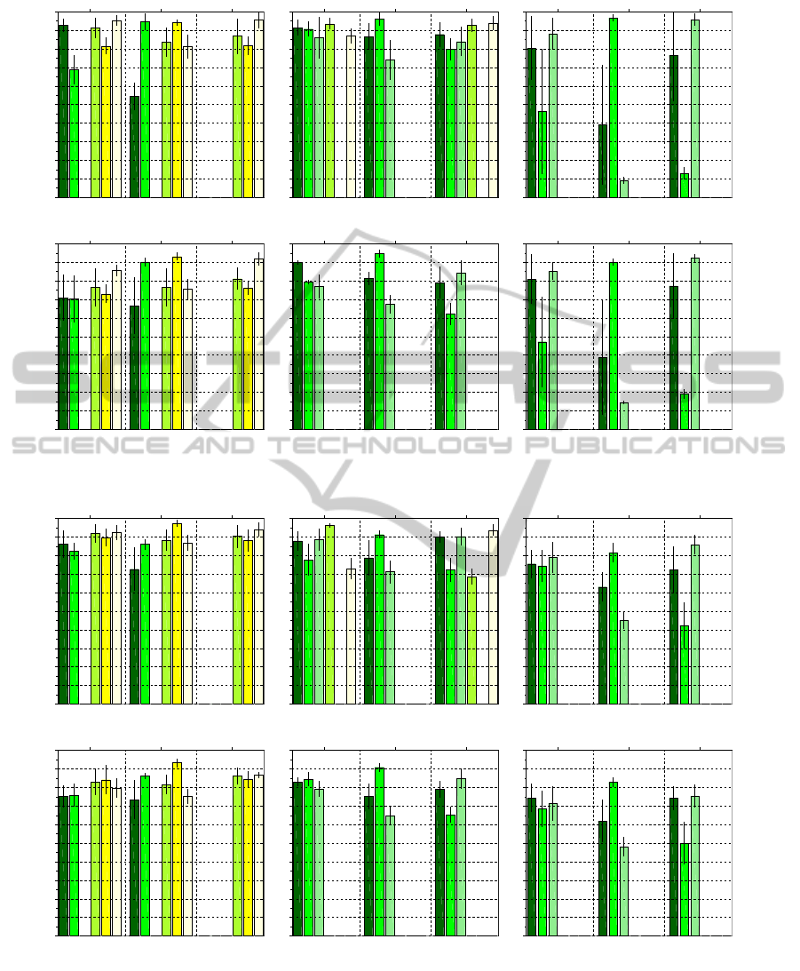
Figure 1 shows the best results obtained for the GIST
and CENTRIST descriptors. Those results were ob-
tained with the SOM size fixed to S = 20 × 20 and
using an infinite integration window.
The overall results are good. For instance, the av-
erage recognition rate when trained and tested under
the same illumination condition (congruent condition)
can be seen in table 1. Those results are better than the
one described in (Ullah et al., 2008).
Both descriptors show a good robustness to vary-
ing illumination conditions with a slight advantage to
CENTRIST. This can be seen in figure 1: the differ-
ence between classification rates in congruent case, in
one hand, and non-congruent cases, in the other hand,
is smaller for CENTRIST (figure 1(b)) than for GIST
(figure 1(a)).
If we take into consideration all the cases, our sys-
tem performs slightly better for extended sequences
1
See http://cogvis.nada.kth.se/COLD/bugs.php for the
list of erroneous sequences
Table 1: Average recognition rate in congruent conditions
for GIST and CENTRIST descriptors compared to (Ullah
et al., 2008). For each laboratory, the best result is in bold.
The results show that GIST performs slightly better than
CENTRIST especially in Ljubljana.
GIST CENTRIST (Ullah et al., 2008)
Saar. - Std 93.7% 91.1% 90.5%
Saar. - Ext 84.5% 84.9% 83.8%
Frei.- Std 91.7% 91.9% 85.6%
Frei.- Ext 89.6% 86.2% 81.8%
Ljub. - Std 90.7% 81.0% 90.4%
Ljub. - Ext 87.7% 77.6% 85.5%
but slightly less well than the one described in (Ullah
et al., 2008) for standard sequences. A notable ex-
ception is the Ljubljana laboratory where we perform
less well especially the GIST descriptor on “night”
sequences. A possible explanation is that night se-
quences in the Ljubljana laboratory are very dark. A
global signature is more sensitive to the global illu-
mination level than a local one (such as GIST used
in (Ullah et al., 2008)). For instance the GIST signa-
ture (and the prototypes) for those sequences will be
different from the ones for “sunny” or “cloudy” se-
quences which explains the low recognition rate. As
said previously CENTRIST is more robust to illumi-
nation changes thanks to the CT.
5.3 Influence of the Size of the
Integration Window
The main point of this paper is to study the influence
of the size of the integration window L and possibly
to show a positive impact on performance. To do so
we repeated the experiment above with several val-
ues of L and computed the average recognition rate.
To avoid interaction between the robustness to illumi-
nation and the effect of L we study the case of con-
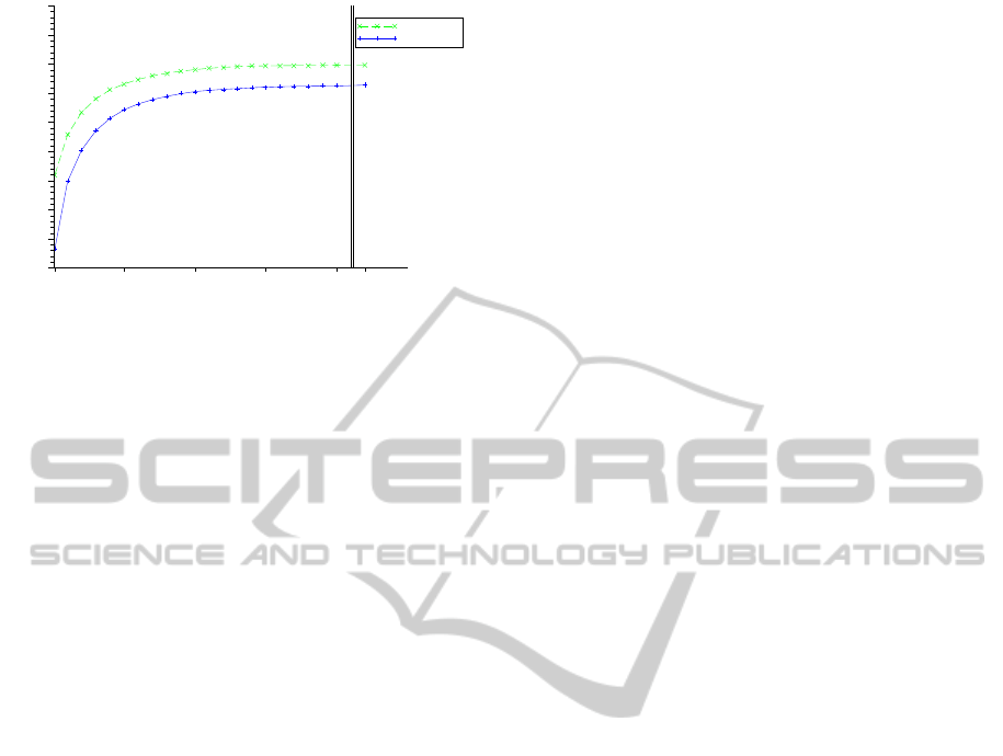
gruent illumination. Figure 2 shows the influence of
the length of the integration window L on the perfor-
mance for each type of signature.
With only one image the system is a pure scene
classification algorithm. The performances are rather
poor (58% of correct recognition for CENTRIST,
71% for GIST) which suggests that the visual pro-
totypes given by the SOM are not sufficient for place
recognition. The average classification rate increases
quickly as L goes to +∞. For example with GIST
the average performance rises from 71% to nearly
90% (increase of 19%). With CENTRIST the aver-
age recognition rises from 58% to 84% (increase of
26%). With a window of length 50 the average recog-
nition rate is already higher than 80% for CENTRIST
and 85% for GIST.
Given the simplicity of our system which uses
VISAPP 2011 - International Conference on Computer Vision Theory and Applications
290
Std partA: 92.67%
cloudy
Std partA: 54.30%
cloudy
Std partA: 68.82%
night
Std partA: 94.58%
night
Std partB: 91.18%
cloudy
Std partB: 83.62%
cloudy
Std partB: 86.83%
cloudy
Std partB: 81.42%
night
Std partB: 94.13%
night
Std partB: 81.76%
night
Std partB: 95.30%
sunny
Std partB: 81.10%
sunny
Std partB: 95.90%
sunny
Saarbruecke n - Std
0.0
0.1
0.2
0.3
0.4
0.5
0.6
0.7
0.8
0.9
1.0
cloudy night sunny
Ext partA: 70.87%
cloudy
Ext partA: 66.49%
cloudy
Ext partA: 70.14%
night
Ext partA: 90.15%
night
Ext partB: 76.37%
cloudy
Ext partB: 76.43%
cloudy
Ext partB: 81.14%
cloudy
Ext partB: 72.95%
night
Ext partB: 93.10%
night
Ext partB: 76.20%
night
Ext partB: 85.51%
sunny
Ext partB: 75.58%
sunny
Ext partB: 91.93%
sunny
Saarbruecke n - Ext
0.0
0.1
0.2
0.3
0.4
0.5
0.6
0.7
0.8
0.9
1.0
cloudy night sunny
Std partA: 91.35%
cloudy
Std partA: 86.63%
cloudy
Std partA: 87.74%
cloudy
Std partA: 90.61%
night
Std partA: 96.03%
night
Std partA: 79.70%
night
Std partA: 85.90%
sunny
Std partA: 73.95%
sunny
Std partA: 83.93%
sunny
Std partB: 93.46%
cloudy
Std partB: 92.63%
cloudy
Std partB: 86.88%
sunny
Std partB: 93.97%
sunny
Freiburg - St d
0.0
0.1
0.2
0.3
0.4
0.5
0.6
0.7
0.8
0.9
1.0
cloudy night sunny
Ext partA: 89.79%
cloudy
Ext partA: 81.37%
cloudy
Ext partA: 78.94%
cloudy
Ext partA: 79.26%
night
Ext partA: 94.62%
night
Ext partA: 62.17%
night
Ext partA: 76.99%
sunny
Ext partA: 67.53%
sunny
Ext partA: 84.42%
sunny
Freiburg - Ext
0.0
0.1
0.2
0.3
0.4
0.5
0.6
0.7
0.8
0.9
1.0
cloudy night sunny
Std partA: 80.34%
cloudy
Std partA: 39.05%
cloudy
Std partA: 76.58%
cloudy
Std partA: 46.44%
night
Std partA: 96.64%
night
Std partA: 12.93%
night
Std partA: 88.12%
sunny
Std partA: 9.27%
sunny
Std partA: 95.61%
sunny
Ljubljana - Std
0.0
0.1
0.2
0.3
0.4
0.5
0.6
0.7
0.8
0.9
1.0
cloudy night sunny
Ext partA: 80.80%
cloudy
Ext partA: 38.55%
cloudy
Ext partA: 77.22%
cloudy
Ext partA: 47.13%
night
Ext partA: 90.01%
night
Ext partA: 19.23%
night
Ext partA: 85.02%
sunny
Ext partA: 14.51%
sunny
Ext partA: 92.25%
sunny
Ljubljana - Ext
0.0
0.1
0.2
0.3
0.4
0.5
0.6
0.7
0.8
0.9
1.0
cloudy night sunny
(a) GIST
Std partA: 86.14%
cloudy
Std partA: 72.59%
cloudy
Std partA: 82.24%
night
Std partA: 86.03%
night
Std partB: 92.02%
cloudy
Std partB: 88.15%
cloudy
Std partB: 90.38%
cloudy
Std partB: 89.68%
night
Std partB: 97.18%
night
Std partB: 87.98%
night
Std partB: 92.39%
sunny
Std partB: 86.65%
sunny
Std partB: 93.96%
sunny
Saarbruecke n - Std
0.0
0.1
0.2
0.3
0.4
0.5
0.6
0.7
0.8
0.9
1.0
cloudy night sunny
Ext partA: 75.17%
cloudy
Ext partA: 73.38%
cloudy
Ext partA: 75.71%
night
Ext partA: 86.30%
night
Ext partB: 82.90%
cloudy
Ext partB: 81.60%
cloudy
Ext partB: 86.21%
cloudy
Ext partB: 84.15%
night
Ext partB: 93.30%
night
Ext partB: 84.45%
night
Ext partB: 79.78%
sunny
Ext partB: 75.32%
sunny
Ext partB: 86.83%
sunny
Saarbruecke n - Ext
0.0
0.1
0.2
0.3
0.4
0.5
0.6
0.7
0.8
0.9
1.0
cloudy night sunny
Std partA: 87.81%
cloudy
Std partA: 78.71%
cloudy
Std partA: 89.99%
cloudy
Std partA: 77.68%
night
Std partA: 91.25%
night
Std partA: 72.20%
night
Std partA: 88.58%
sunny
Std partA: 71.21%
sunny
Std partA: 90.32%
sunny
Std partB: 96.27%
cloudy
Std partB: 68.65%
cloudy
Std partB: 72.80%
sunny
Std partB: 93.65%
sunny
Freiburg - St d
0.0
0.1
0.2
0.3
0.4
0.5
0.6
0.7
0.8
0.9
1.0
cloudy night sunny
Ext partA: 83.04%
cloudy
Ext partA: 75.12%
cloudy
Ext partA: 79.00%
cloudy
Ext partA: 84.33%
night
Ext partA: 90.86%
night
Ext partA: 65.23%
night
Ext partA: 79.26%
sunny
Ext partA: 64.55%
sunny
Ext partA: 84.65%
sunny
Freiburg - Ext
0.0
0.1
0.2
0.3
0.4
0.5
0.6
0.7
0.8
0.9
1.0
cloudy night sunny
Std partA: 75.47%
cloudy
Std partA: 63.00%
cloudy
Std partA: 72.29%
cloudy
Std partA: 74.43%
night
Std partA: 81.64%
night
Std partA: 42.30%
night
Std partA: 78.93%
sunny
Std partA: 44.88%
sunny
Std partA: 85.80%
sunny
Ljubljana - Std
0.0
0.1
0.2
0.3
0.4
0.5
0.6
0.7
0.8
0.9
1.0
cloudy night sunny
Ext partA: 74.33%
cloudy
Ext partA: 61.91%
cloudy
Ext partA: 74.25%
cloudy
Ext partA: 68.38%
night
Ext partA: 82.87%
night
Ext partA: 49.86%
night
Ext partA: 71.51%
sunny
Ext partA: 48.06%
sunny
Ext partA: 75.45%
sunny
Ljubljana - Ext
0.0
0.1
0.2
0.3
0.4
0.5
0.6
0.7
0.8
0.9
1.0
cloudy night sunny
(b) CENTRIST
Figure 1: An example of performance of our system in place recognition task: (a) for the GIST descriptor (b) for the CEN-
TRIST descriptor. The uncertainties are given as one standard deviation. Missing bars represent missing data. The laboratory
and part are shown under the graph. The top row shows results for standard sequences and the bottom row for extended
sequences. The illumination condition used for training is shown on top of each figure. The illumination condition used
for testing is shown under each bar. The part of the laboratory is shown inside the bar. The vertical axes is the average
classification rate.
TEMPORAL BAG-OF-WORDS - A Generative Model for Visual Place Recognition using Temporal Integration
291
GIST
CENTRIST
0.55
0.60
0.65
0.70
0.75
0.80
0.85
0.90
0.95
1.00
1 50 100 150 200 Inf
Length of the integration window (step)
Average recognition rate (%)
Figure 2: Influence of the size of the integration window on
the average classification rate for each signature.
only a global and very coarse description of each
scene this demonstrates the benefits of temporal in-
tegration for place recognition.
6 CATEGORIZATION
OF PLACES
In this experiment we test the system on a place cate-
gorization task. Place categorization is a much harder
task because the goal is to assign the label “office” to
any office in the test set while the system has been
trained on other offices. Therefore it is interesting to
assess the performance of our system on such a task
and to study the influence of the parameters.
Again, for fair comparison, we reproduce the ex-
perimental design of (Ullah et al., 2008). Here the
algorithm is trained to recognize four different room
categories (corridor, printer area, two-persons office
and bathroom), all available in the standard sequences
of part “A” of each laboratory. The algorithm is
trained on two sequences taken from two laborato-
ries. Testing was performed on sequences taken at the
third remaining laboratory. In this case the training
and testing illumination condition are the same.
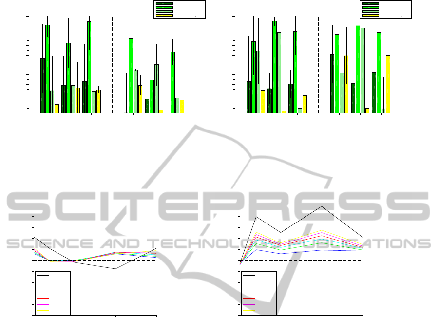
Figure 3 shows results obtained for the 2 signa-
tures with a SOM size of S = 5 × 5 for GIST and
15 ×15 for CENTRIST. In both cases we used an in-
finite integration window.
Like in (Ullah et al., 2008) the corridor is al-
ways the best recognized category but CENTRIST
also performed well on the two-persons office. Av-
eraged across all the tests CENTRIST achieve classi-
fication rates of 84.72% for the corridor, 47.96% for
the two-persons office, 37.16% for the printer area
and 28.18% for the bathroom. The performances of
GIST are 72.21%, 30.95%, 22.12% and 17.67% re-
spectively.
Those results are better than those reported in (Ul-
lah et al., 2008) (76.73% for the corridor, far lower for
other places). (Wu et al., 2009) obtained interesting
results but on a different dataset.
To evaluate the influence of the two parameters S
and L we performed the same experiment for S rang-
ing from 5×5 to 20×20 and L ranging from 1 to +∞.
To assess the system we use the average recognition
rate.
Figure 4 shows the results for the 2 descriptors.
GIST didn’t perform well on this categorization task:
the responses are barely above the level of chance
(25% since we have 4 categories). This result is
coherent with the low performances of GIST in in-
door scene categorization task (see (Quattoni and Tor-
ralba, 2009)). As CENTRIST was designed for place
categorization we expected good results for this de-
scriptor: the average recognition rate reaches 50%
for S = 15 and infinite integration window which is
higher than the results reported in (Ullah et al., 2008).
Interestingly, unlike the case of recognition, the
effect of the size of the SOM is non-monotonic.
This may be explained by the fact that on one hand
a smaller SOM implies less visual prototypes and
then may ease categorization but on the other hand a
smaller SOM decreases the ability to discriminate be-
tween different rooms which may lead to confusion
between different categories.
The effect of L on this task is clear for CEN-
TRIST: a larger window always give better results
which shows the interest of our integration method.
However a closer look at data shows that there is a
high false-positive rate. In fact the high classification
rate can be explained because one or two classifiers
win most of the time (the classifiers for the toilets and
the corridor in our case). This also explains the large
deviation that we observe.
7 CONCLUSIONS
The main contribution of this paper is to show the
advantage of temporal integration of visual cues for
place recognition. This idea is deeply linked with the
spatial nature of a place and the abilities of a robot
to explore it. It allows to describe the visual environ-
ment in terms of global content while keeping good
recognition rate and can be used for different systems.
We have presented a BoW-like system that takes
advantage of this approach in several ways. Visual en-
vironment can be described thanks to coarse descrip-
tors and a small number of visual prototypes based
on global features (i.e. a dictionary of visual scenes).
Combined with cue integration they form a genera-
VISAPP 2011 - International Conference on Computer Vision Theory and Applications
292
Printer Area
Corridor
2 Persons Office
Bathroom
Training condition
cloudy night
0.0
0.1
0.2
0.3
0.4
0.5
0.6
0.7
0.8
0.9
1.0
Saar Ljub Freib Saar Ljub Freib
Recognition laboratory
Average recognition rate (%)
(a) GIST
Printer Area
Corridor
2 Persons Office
Bathroom
Training condition
cloudy night
0.0
0.1
0.2
0.3
0.4
0.5
0.6
0.7
0.8
0.9
1.0
Saar Ljub Freib Saar Ljub Freib
Recognition laboratory
Average recognition rate (%)
(b) CENTRIST
Figure 3: Example of results obtained (a) with GIST and a SOM of size S = 5 × 5 (b) with CENTRIST and a SOM of
S = 15 × 15. In both cases we used an infinite integration window. The uncertainties are given as one standard deviation. The
illumination condition used for training and testing is shown on top of the figure. The laboratory used for training is shown
under.
Infinity
1
10
20
30
40
50
0.00
0.05
0.10
0.15
0.20
0.25
0.30
0.35
0.40
0.45
0.50
5 10 15 20
SOM Size
Average perf
(a) GIST
Infinity
1
10
20
30
40
50
0.00
0.05
0.10
0.15
0.20
0.25
0.30
0.35
0.40
0.45
0.50
5 10 15 20
SOM Size
Average perf
(b) CENTRIST
Figure 4: Influence of the size of the SOM and the integration window for signatures computed on the categorization task: (a)
for the GIST descriptor (b) for the CENTRIST descriptor. The line of chance is indicated by the dashed line.
tive, any-time, incremental and on-line place recog-
nition system. The results on the place recognition
task have shown that the system compares well with
state-of-the-art systems. However, despite good per-
formance in some cases, place categorization is still
an open problem.
From a computational point-of-view the most de-
manding phase is the computation of the visual de-
scriptor. CENTRIST is relatively easy to compute.
GIST is more challenging but fast implementation ex-
ists. As the other components of the algorithm are
lightweight we think that our system could be able to
run on real-time on a robotic platform.
The paper also compared two recent descriptors
used for place recognition. GIST gives better results
in the recognition of instances task (despite greater
sensibility to global illumination) while CENTRIST
gives better results for classification.
The average classification rate is a rough metric.
The use of more sophisticated performance measures
like the area under the ROC Curve (which is equiv-
alent to the Wilcoxon test of ranks) could lead to in-
depth inspection of the results.
Future works include a completely on-line algo-
rithm i.e. replacing the SOM with an on-line, incre-
mental algorithm. Several ideas could be used to over-
come the explicit reset during recognition, which is a
clear limitation of the current system. For instance,
we could use a mechanism for detecting doorways.
As we have generative, probabilistic classifiers, we
could also use the uncertainty of the classification to
allow automatic reset.
Our system is compatible with classical BoW
techniques so, to improve the performance and espe-
cially the robustness to illumination, we can use an
interest point based signature like SIFT.
To enforce the independence assumption we
could use subsampling. Alternatively, using n-order
Markov Model (phrases of visual prototypes) may
be interesting because they could capture the time-
TEMPORAL BAG-OF-WORDS - A Generative Model for Visual Place Recognition using Temporal Integration
293

dependence of the visual prototypes during explo-
ration. This would alleviate the independence as-
sumption of our method.
ACKNOWLEDGEMENTS
We thanks David Filliat for fruitful discussion and
code exchange, Mohamed Jaite for setting-up the
COLD database and Andrzej Pronobis for helping us
with the COLD database.
REFERENCES
Csurka, G., Bray, C., Dance, C., and Fan, L. (2004). Visual
categorization with bags of keypoints. In Workshop on
Statistical Learning in Computer Vision, ECCV, pages
1–22.
Douze, M., J
´
egou, H., Sandhawalia, H., Amsaleg, L., and
Schmid, C. (2009). Evaluation of gist descriptors for
web-scale image search. In International Conference
on Image and Video Retrieval. ACM.
Fei-Fei, L. and Perona, P. (2005). A bayesian hierarchi-
cal model for learning natural scene categories. In
IEEE Computer Society Conference on Computer Vi-
sion and Pattern Recognition, volume 2, pages 524–
531.
Filliat, D. (2008). Interactive learning of visual topological
navigation. In Proceedings of the 2008 IEEE Interna-
tional Conference on Intelligent Robots and Systems
(IROS 2008).
Filliat, D. and Meyer, J.-A. (2003). Map-based navigation
in mobile robots - i. a review of localisation strategies.
Journal of Cognitive Systems Research, 4(4):243–282.
Gokalp, D. and Aksoy, S. (2007). Scene classification using
bag-of-regions representations. In IEEE Conference
on Computer Vision and Pattern Recognition (CVPR
2007), pages 1–8, Minneapolis, USA.
Guillaume, H., Denquive, N., and Tarroux, P. (2005). Con-
textual priming for artificial visual perception. In
European Symposium on Artificial Neural Networks
(ESANN 2005), pages 545–550, Bruges, Belgium.
Kohonen, T. (1990). Improved versions of learning vec-
tor quantization. In International Joint Conference on
Neural Networks, pages 545–550.
Lazebnik, S., Schmid, C., and Ponce, J. (2006). Beyond
bags of features: Spatial pyramid matching for rec-
ognizing natural scene categories. In Association, I.,
editor, IEEE Conference on Computer Vision and Pat-
tern Recognition, volume II, pages 2169–2178, New
York.
Mozos, O. M. (2008). Semantic Place Labeling with Mobile
Robots. PhD thesis, University of Freiburg, Freiburg,
Germany.
Mozos, O. M., Stachniss, C., and Burgard, W. (2005). Su-
pervised learning of places from range data using ad-
aboost. In IEEE International Conference on Robotics
and Automation, volume 2.
Ng, A. Y. and Jordan, M. I. (2002). On discriminative
vs. generative classifiers: A comparison of logistic re-
gression and naive bayes. In Advances in Neural In-
formation Processing Systems, volume 14. MIT Press.
Ni, K., Kannan, A., Criminisi, A., and Winn, J. (2009).
Epitomic location recognition. IEEE Transac-
tions on Pattern Analysis and Machine Intelligence,
31(12):2158–2167.
Ojala, T., Pietik
¨
ainen, M., and M
¨
aenp
¨
a
¨
a, T. (2002). Mul-
tiresolution gray-scale and rotation invariant texture
classification with local binary patterns. IEEE Trans-
actions on Pattern Analysis and Machine Intelligence,
pages 971–987.
Oliva, A. and Torralba, A. (2001). Modeling the shape
of the scene: A holistic representation of the spatial
envelope. International Journal of Computer Vision,
42(3):145–175.
Orabona, F., Castellini, C., Caputo, B., Luo, J., and Sandini,
G. (2007). Indoor place recognition using online in-
dependent support vector machines. In Proceeding of
the British Machine Vision Conference (BMVC 2007),
pages 1090–1099, Warwick, UK.
Pronobis, A. and Caputo, B. (2007). Confidence-based cue
integration for visual place recognition. In Proceed-
ings of the IEEE/RSJ International Conference on In-
telligent Robots and Systems (IROS 2007), San Diego,
CA, USA.
Pronobis, A. and Caputo, B. (2009). Cold: Cosy localiza-
tion database. The International Journal of Robotics
Research, 28(5).
Pronobis, A., Caputo, B., Jensfelt, P., and Christensen, H. I.
(2006). A discriminative approach to robust visual
place recognition. In Proceedings of the IEEE/RSJ In-
ternational Conference on Intelligent Robots and Sys-
tems (IROS 2006), pages 3829–3836, Beijing, China.
Pronobis, A., Mozos, O. M., Caputo, B., and Jenseflt, P.
(2010). Multi-modal semantic place classification.
The International Journal of Robotics Research, 29(2-
3):298–320.
Quattoni, A. and Torralba, A. (2009). Recognizing indoor
scenes. In IEEE Conference on Computer Vision and
Pattern Recognition.
Torralba, A. (2003). Contextual priming for object de-
tection. International Journal of Computer Vision,
53(2):169–191.
Torralba, A., Murphy, K., Freeman, W., and Rubin, M.
(2003). Context-based vision system for place and ob-
ject recognition. Technical report, Cambridge, MA.
Ullah, M. M., Pronobis, A., Caputo, B., Luo, J., Jensfelt, P.,
and Christensen, H. I. (2008). Towards robust place
recognition for robot localization. In Proceedings of
the IEEE International Conference on Robotics and
Automation (ICRA 2008), Pasadena, USA.
VISAPP 2011 - International Conference on Computer Vision Theory and Applications
294

Vasudevan, S. and Siegwart, R. (2008). Bayesian space
conceptualization and place classification for seman-
tic maps in mobile robotics. Robotics and Autonomous
Systems, 56(6):522–537.
Walker, L. and Malik, J. (2004). When is scene identi-
fication just texture recognition? Vision Research,
44:23012311.
Wu, J., Christensen, H., and Rehg, J. (2009). Visual
place categorization: Problem, dataset, and algorithm.
In IEEE/RSJ International Conference on Intelligent
Robots and Systems, 2009 (IROS 2009), pages 4763–
4770, St. Louis, USA. IEEE.
TEMPORAL BAG-OF-WORDS - A Generative Model for Visual Place Recognition using Temporal Integration
295
