
AN APPROXIMATION OF GAUSSIAN PULSES
Sorin Pohoaţă
Department of Computer and Automation, “Ştefan cel Mare” University of Suceava
str. Universităţii, no.13, RO-720225 Suceava, Romania
Nicolae Dumitru Alexandru, Adrian Popa
Department of Telecommunications, “Gh. Asachi” Technical University of Iaşi
Bd. Carol I, no.11, RO-700506 Iaşi, Romania
Keywords: Ultra wide-band, Impulse radio.
Abstract: A new technique for generating an approximate replica of Gaussian pulses with good accuracy is proposed
and investigated. The Gaussian function is approximated with a waveform that results from the convolution
of two triangles. The proposed pulse performs better than other previously reported pulse. The results show
good agreement not only for the Gaussian pulse but also for its first and second derivatives. As the
triangular pulse generator is standard and widely used, the proposed technique needs besides it an
appropriate filter.
1 INTRODUCTION
Gaussian pulses are widely used in communications,
as they show maximum steepness of transition with
no overshoot and minimum group delay. Several
applications are mobile telephony (GSM) where
Gaussian Minimum Shift Keying (GMSK) signals
are used and ultra-wideband (UWB)
communications, where ultra-short pulses based on
the Gaussian shape are generated.
The Ultra-wideband (UWB) technology
(Guofeng, 2003)(Xiliang, 2003) is a new technology
for short range, high data rate wireless
communication and it was investigated for use in
high data-rate indoor wireless networks. UWB can
also be used for Personal Area Networks (PAN) as it
can deliver data speeds of 480 Mbps at distances of
2-3 meters. A UWB
communication system
transmits pulses which occupy several GHz of
spectrum (from near DC).
As it occupies a very large bandwidth, UWB
technology is subjected to very strict spectral and
power constraints in order to coexist with other
existing communication systems. There are stringent
regulations on the radiated energy in order to avoid
interference, set by the Federal Communications
Commission (FCC) (FCC, 2002). As a consequence,
the spectral shape of UWB signals is an important
implementation aspect, adhering to constraints and
still maximizing available signal power, to enable
the targeted high data rate applications (Guofeng,
2003). One should maximize the total transmitted
power across the band while complying with the
imposed spectral mask.
If the spectral properties are not optimized, the
output power has to be lowered to fulfil the mask
requirements in every frequency band. Since the
ultra-short pulses used are generated with analog
components, e.g., the Gaussian Monocycle, their
spectral shape is not easy to design. Replacing the
analog pulses with digital designs is prohibited by
the huge bandwidth and the resulting sampling rates
(Berger, 2006).
The most frequently used pulse signals in digital
communications are:
1. rectangular pulse;
2. cosine pulse (MSK);
3. raised cosine pulse (quadrature overlapped
raised-cosine - QORC);
4. Gaussian pulse (GMSK, UWB).
A Gaussian pulse is a good choice of shaping
function since it provides a particularly compact
frequency domain spectrum. In general the
improvement stems from the elimination of the
broad pattern of side lobes characteristic of a
359
Pohoa¸t
ˇ
a S., Dumitru Alexandru N. and Popa A..
AN APPROXIMATION OF GAUSSIAN PULSES.
DOI: 10.5220/0003357203590364
In Proceedings of the 1st International Conference on Pervasive and Embedded Computing and Communication Systems (PECCS-2011), pages
359-364
ISBN: 978-989-8425-48-5
Copyright
c
2011 SCITEPRESS (Science and Technology Publications, Lda.)

rectangular pulse, which extends to a surprisingly
large distance from the centre frequency (Berger,
2006)(Dou, 2000).
The frequency-domain representation and
Fourier transform of the Gaussian pulse are:
2
2
2σ
f
e
σ2π
1
H(f)
−
⋅=
(1)
222
tσπ2
eσπ2h(t)
−
=
(2)
A true Gaussian pulse has theoretically an
infinite extent, so, one has to truncate the tails in
time domain and investigate the consequences in the
frequency domain. In GMSK the pre-modulation
filter is Gaussian and has a transfer function
2
2ln
2
eH(f)
⋅
⎟
⎠
⎞
⎜
⎝
⎛
−
⋅=
B
f
A
(3)
where B is the 3 dB band of the filter and A is a
constant. If,
B
0.5887
B2
ln2
α ==
(4)
the impulse response of the filter becomes
2
2
2
t
α
π
e
α
π
h(t)
⋅−
⋅=
(5)
In GMSK the Gaussian filter makes smooth the
phase trajectory of the MSK signal and limits the
variations of the instantaneous frequency of the
signal. The impulse response of the filter to a
rectangular signal of duration T is (Murota, 1981)
dueTB
ln2
2π
A(t)g
1/2t/T
1/2t/T
ln2
uT)(B2π
s
222
∫
+
−
⋅⋅
−
⋅⋅⋅=
(6)
It can also be expressed as equation (7):
⎭
⎬
⎫
⎩
⎨
⎧
⎥
⎦
⎤
⎢
⎣
⎡
⎟
⎠
⎞
⎜
⎝
⎛
−−
⎥
⎦
⎤
⎢
⎣
⎡
⎟
⎠
⎞
⎜
⎝
⎛
+⋅=
2
T
tcBerf
2
T
tcBerfK(t)g
s
(7)
or
⎥
⎦
⎤
⎢
⎣
⎡
⎟
⎠
⎞
⎜
⎝
⎛
+
−
⎟
⎠
⎞
⎜
⎝
⎛
−
⋅=
ln2
T/2t
B2πQ
ln2
T/2t
B2πQ
2T
1
(t)g
s
(8)
where K is a constant chosen in order that the
area of the impulse be equal to
1/ 2
, c is a constant
2/ln2πc =
and B is the 3 dB bandwith.
In the sequel we will concentrate on obtaining a
good approximation of the Gaussian pulse and its
first derivative.
2 FREQUENCY SPECTRUM
A frequently used signalling waveform in digital
communication is the rectangular pulse, as it can be
produced easily, even at high speeds. However, the
rectangular pulse shows a power spectrum that
decays slowly.
The power spectral density (p.s.d.) of a polar
NRZ-L transmission using equiprobable data bits
(
501 .pp
=
−
=
) (Bennett, 1958), is given by
2
G(f)
T
1
W(f) =
(9)
where G(f) denotes the Fourier transform of the
signaling pulse g(t), and T is the duration of the bit
interval.
The rectangular pulse of amplitude A and
duration T has a Fourier transform
0
f/fπ
)
0
f/fsin(π
AT
fTπ
fTsinπ
ATG(f) ⋅=⋅=
(10)
where
Tf /1
0
=
is the signalling frequency (data rate)
and
0
/ ff
is the normalized frequency with respect
to the data rate. The Fourier transform decays rather
slowly as
f/1
, taking into account the
discontinuous character of the signalling waveform
(rectangular pulse). As a consequence, its p.s.d. will
decay as
2−
f
.
A well-known theorem in the theory of Fourier
transform states that if the signalling waveform
)(tg
is continuous and equal to zero at the ends of the
signalling interval (
2/T
±
), and has a number of
1
−
k
derivatives that are continuous and equal to
zero at the ends of the signalling interval, then the
Fourier transform will decay as
)1( +− k
f
(Beaulieu,
2004)(Alexandru, 2009). Accordingly, the p.s.d. will
decay as
)1(2 +− k
f
. We will denote this as the
continuity feature of
thk −
−
)1(
order.
Let us consider a raised cosine (RC) pulse
described by equation (11):
()
⎪
⎩
⎪
⎨
⎧
≤+
=
elsewhere0
2
T
tt2πcos1
2
1
g(t)
(11)
It satisfies
0g(t)
T/2t
=
±=
(12)
Its first derivative is
0tsin2ππ(t)g
T/2t
=−=
′
±=
(13)
PECCS 2011 - International Conference on Pervasive and Embedded Computing and Communication Systems
360

As
0(t)g
T/2t
≠
′′
±=
(14)
the signalling pulse g(t) has
11 =−k
derivatives that
are continuous and equal to zero at the ends of the
signalling interval (
2/T±
), k = 2 and the p.s.d. will
decay as
6−
f
, as seen in Figure 1 in comparison
with the spectrum of a rectangular pulse that decays
as
2−
f
.
Figure 1: Power spectral density of rectangular and RC
pulse.
The Fourier transform of g(t) is given by
)
2
T
2
f(1fπ
fTsinπ
2
1
G(f)
−
=
(15)
The RC pulse with a width
T results from the
convolution of a rectangular pulse of width
T/2 with
a cosine lobe of width
T/2.
3 PULSES RESULTED FROM
CONVOLUTION
To exhibit better spectral properties the signalling
waveform
g(t) should be continuous and equal to
zero at the ends of the signalling interval (
2/T
±
)
and possess a large number of derivatives that are
continuous and equal to zero at the ends of the
signalling interval.
This condition is easily met if the signalling pulses
are obtained as a result of convolution. Let us
assume that a pulse
g(t) is obtained from the
convolution of two pulses
x(t) and y(t)
∫
−=∗= τ)y(τ)dτx(ty(t)x(t)g(t)
(16)
Y(f)X(f)G(f)
⋅
=
(17)
If
x(t) and y(t) possess continuity of
thk
−
−
)1(
and
thl −− )1(
order, respectively, then the p.s.d. of
G(f) will show a fast roll-off proportional to
)2(2 ++− lk
f
, which corresponds to a
thlk −+ )(
order
of continuity.
As an example let us consider the RC pulse given
by equation (18):
()
⎪
⎩
⎪
⎨
⎧
≤+
=
elsewhere0
Ttt/Tcos(π1
2
1
g(t)
(18)
which results from the convolution of a rectangular
pulse with a cosine pulse, both of duration
T. The
resulted pulse has duration of 2
T. In Figure 1 we
represented the p.s.d. for a rectangular and a RC
pulse. As seen, the spectral roll-off rate is bigger for
RC pulse, as it exhibits better continuity properties.
We shall characterize a pulse signalling waveform
by
CnDm; n = 0, 1 and m = 0, 1, 2, 3, …
n=0 means that the signalling waveform is not
continuous and equal to zero at the ends of the
signalling interval and
n=1 denotes the opposite.
m is the number of the derivatives that satisfy the
m-th order of continuity condition.
A rectangular pulse can be characterized as
C0D0 and a cosine pulse as C1D0. The RC pulse
that results from their convolution is described by
C1D1. A few classes of signalling pulses are
described in Table 1.
Table 1: Classes of signalling pulses produced by
convolution.
I x(t) II y(t) III x(t)*y(t)
C
0
D
0
Rectangle
C
0
D
0
Rectangle
C
1
D
0
Triangle
C
0
D
0
Rectangle
C
1
D
0
Triangle
Cosine lobe
C
1
D
1
C
1
D
1
Raised cosine
C
0
D
0
Rectangle
C
1
D
1
Raised cosine
C
1
D
2
C
1
D
0
Triangle
Cosine lobe
C
1
D
0
Triangle
Cosine lobe
C
1
D
2
C
1
D
0
Triangle
Cosine lobe
C
1
D
1
Raised cosine
C
1
D
3
C
1
D
1
Raised cosine
C
1
D
1
Raised cosine
C
1
D
4
C
1
D
1
Raised cosine
C
1
D
2
Cos*Cos
C
1
D
5
C
1
D
1
Raised cosine
C
1
D
4
Rcos*Rcos
C
1
D
7
C
1
D
2
Cos*Cos
C
1
D
2
Cos*Cos
C
1
D
6
AN APPROXIMATION OF GAUSSIAN PULSES
361
4 APPROXIMATIONS
OF GAUSSIAN PULSE
An approximation of Gaussian pulse in the interval
)3,3(−
(Dimitrov, 1991) used the method of linear
voltage integration. The Gaussian function was
approximated for
1=
σ
and was normalized to
obtain
.1)0( =h
The Gaussian characteristic is
replaced by a piece-wise parabolic approximation
using polynomials of power 2 (quadratic parabolas)
of the type:
2
n2n10
xcxccy(t) ++=
(19)
where
n
x
is a discrete variable. When
n
x
changes
gradually during the calculations with a step of 0.01
,
(Dimitrov, 1991) the approximation function that
minimizes the relative error of approximation is
given by the reunion of three parabolic pieces, as
⎪
⎪
⎩
⎪
⎪
⎨
⎧
≤≤+−
≤≤−−
−≤≤−++
=
elsewhere
xxx
xx
xxx
xy
,0
31,1472.08848.03276.1
11,40548.099089.0
13,1472.08848.03276.1
)(
2
2
2
(20)
5 PROPOSED SOLUTION
By convolving a rectangular pulse of width T with
itself, a triangular pulse of width 2
T is obtained. We
shall use the waveforms resulting from the
convolutions of triangular waveforms defined by
⎪
⎪
⎩
⎪
⎪
⎨
⎧
∈
⎟
⎠
⎞
⎜
⎝
⎛
−
−∈
⎟
⎠
⎞
⎜
⎝
⎛
+
=
T][0,t
T
t
1
0]T,[t
T
t
1
T)g(t,
(21)
The convolution of two triangles of width 2
T,
which is equivalent to convolving four rectangular
pulses of width
T (Alexandru, 1998), results in an
impulse of width 4
T, which is defined by
⎪
⎪
⎪
⎩
⎪
⎪
⎪
⎨
⎧
≤≤
⎟
⎟
⎠
⎞
⎜
⎜
⎝
⎛
−
≤≤−
⎟
⎟
⎟
⎠
⎞
⎜
⎜
⎜
⎝
⎛
⎟
⎟
⎠
⎞
⎜
⎜
⎝
⎛
+
⎟
⎠
⎞
⎜
⎝
⎛
−
==
2TtT
T
t
2
6
T
TtT
T
t
2
1
T
t
3
2
T
T)g(t,*T)g(t,T)s(t,
3
3
2
(22)
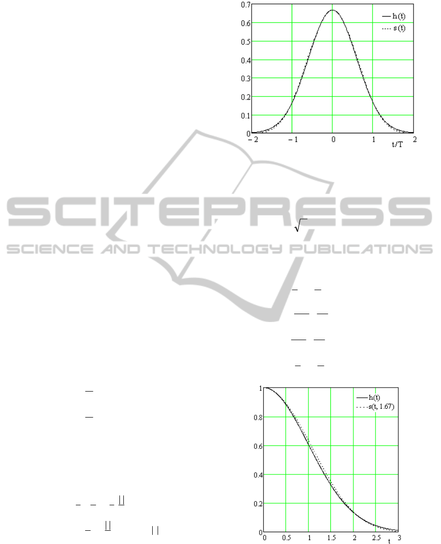
Figure 2 displays the
s(t) waveform together with
a Gaussian pulse with mean value 0 and dispersion
0.266
σ
= . The resemblance is obvious. Figure 3
illustrates the Gaussian pulse with
1=
σ
and its
approximation
),( Tts
with T=1.67.
Figure 2: Gaussian pulse h(t) with
266.0=
σ
and its
approximation s(t) with T = 1.
The first derivative of the Gaussian pulse is
given by:
222
tσπ25/23
eπtσ24(t)h'
−
−=
(23)
The first derivative of
s(t) pulse is given by
equation (24):
⎪
⎪
⎪
⎪
⎪
⎩
⎪
⎪
⎪
⎪
⎪
⎨
⎧
≤≤
⎟
⎠
⎞
⎜
⎝
⎛
−−
≤≤
⎟
⎟
⎠
⎞
⎜
⎜
⎝
⎛
−
≤≤−
⎟
⎟
⎠
⎞
⎜
⎜
⎝
⎛
+−
≤≤−
⎟
⎠
⎞
⎜
⎝
⎛
+
=
′
2TtT
T
t
2
2
1
Tt0T
T
2t
2T
3t
0tTT
T
2t
2T
3t
Tt2T
T
t
2
2
1
T)(t,s
2
23
2
23
2
2
(24)
Figure 3: Normalized Gaussian pulse h(t) with
1
=
σ
and
its approximation s(t, T) with T = 1.67.
Figure 4 illustrates the first derivatives of the
Gaussian pulse and of its approximation
(t)s'
.
PECCS 2011 - International Conference on Pervasive and Embedded Computing and Communication Systems
362
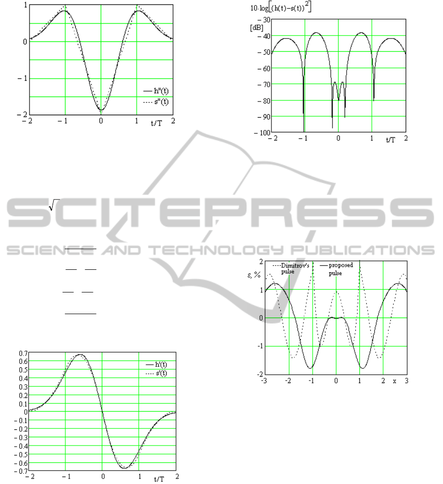
Figure 4: First order derivatives of Gaussian pulse h(t) for
266.0=
σ
and its approximation s’(t).
The second derivative of Gaussian pulse h(t) is
given by equation (25):
()
1tσπ4eπσ24(t)h
222tσπ25/23
222
−=
′′
−
(25)
and
()
()
⎪
⎪
⎪
⎪
⎩
⎪
⎪
⎪
⎪
⎨
⎧
≤≤
−
≤≤
⎟
⎠
⎞
⎜
⎝
⎛
−
≤≤−
⎟
⎠
⎞
⎜
⎝
⎛
+−
≤≤−
+
=
′
2TtT
/2
Tt0T
T
2
T
3t
0tTT
T
2
T
3t
Tt2T
/2
T)(t,s
23
23
T
Tt
T
Tt
(26)
They are illustrated in Figure 5.
Figure 5: Second order derivatives of Gaussian pulse h(t)
for
0.266σ =
and its approximation s”(t).
The squared value of the approximation error:
(
)
2
2
h(t)s(t)(t)e −=
(27)
is illustrated in Figure 6 in logarithmic
representation for
T = 1 and
0.266σ =
and proves to
be quite small.
Figure 6: Mean square value of the approximation error in
logarithmic representation.
Figure 7 illustrates the relative error of
approximation for Dimitrov’s pulse and the
proposed pulse, for which
t/T was substituted by x.
One can see that the proposed pulse performs better
than the Dimitrov’s pulse.
Figure 7: Relative error of approximation.
6 CONCLUSIONS
An approximation of the Gaussian pulse based on a
waveform resulted from the convolution of four
rectangles or equivalently of two triangles was
proposed. A closed-form expression was derived for
it implying polynomials of third degree in
t.
The relative approximation error is quite small,
so this makes it a good substitute for the Gaussian
pulse. A better performance was obtained with
respect to other proposed approximation (Dimitrov,
1991). This technique can be used for generation of
Gaussian pulses in communication systems. As the
triangular pulse generator is standard and widely
used, the proposed technique needs besides it an
appropriate filter.
AN APPROXIMATION OF GAUSSIAN PULSES
363

ACKNOWLEDGEMENTS
This paper was supported by the project "Progress
and development through post-doctoral research and
innovation in engineering and applied sciences -
PRiDE - Contract no. POSDRU/89/1.5/S/57083",
project co-funded from European Social Fund
through Sectorial Operational Program Human
Resources 2007-2013.
REFERENCES
Alexandru, N. D, Davideanu, C., Cehan, V., Scripcariu,
L., Păncescu, L., 1998. On a Class of Continous Pulse
Shapes. In ICT’98, Porto Carras, Greece, June vol. I,
pp. 208-212.
Alexandru, N. D., Pohoaţă, S., 2009. Improved Nyquist
Filters with a Transfer Characteristic Derived from a
Staircase Characteristic Interpolated with Sine
Functions. In Advances in Electrical and Computer
Engineering, vol.9, No.2, Suceava, Romania, pp.103-
108.
Beaulieu, N. C., Damen, M. O., 2004. Parametric
construction of Nyquist-I pulses. In IEEE Trans.
Commun., Vol. 52, pp.2134-2142.
Bennett, W. R., 1958. Statistics of Regenerative Digital
Transmission. In Bell System Techn. J., Vol. 37,
pp.1501-1542.
Berger, C. R., Eisenacher, M., Jäkel, H., Jondral F., 2006.
Pulse Shaping In UWB Systems Using Semidefinite
Programming with Non-Constant Upper Bounds. In
PIMRC’06, http://www.ece.cmu.edu/~crberger.
Dimitrov, J., 1990. A bell-shape pulse generator. In IEEE
Trans. on Instrumentation and Measurement; Vol.39,
No.4, pp.667–670
Dou, W. B., Yung, E. K. N., 2000. Spectrum
transformation of Gaussian Pulse in Waveguide by
FDTD and its Effect on Analysis of Discontinuity
Problem. In Intern. Journal of Infrared and Millimeter
Waves, Vol. 21, No.7, pp.1131-1139.
FCC, 2002. In the matter of revision of part 15 of the
commission’s rules regarding ultra-wideband
transmission systems. In Federal Communications
Commission, First Report and Order
Lu, G., Spasojevic, P., Greenstein, L., 2003. Antenna and
Pulse Designs for Meeting UWB Spectrum Density
Requirements. In IEEE Conf. on Ultra Wideband
Systems and Technologies, pp.162 – 166.
Luo, X., Yang, L., Giannakis, G. B., 2003. Designing
Optimal Pulse-Shapers for Ultra-Wideband Radios. In
Journal of Communications and Networks, Vol. 5, No.
4, pp.344-353.
Murota, K. and Hirade, K., “GMSK Modulation for
Digital Mobile Radio Telephony”, In IEEE Trans.
Communications, Vol. COM-29, pp. 1044 – 1050, July
1981.
Zhang, X., Elgamel, M., Bayoumi, M., Gaussian pulse
approximation using standard CMOS and its
application for sub-GHz UWB impulse radio. In
International Journal of Circuit Theory and
Applications, Vol.38, Issue 4, pp. 383-407, 2010
Wentzloff, D. D., Chandrakasan, A. P., Gaussian pulse
generators for subbanded ultra wideband transmitters.
In IEEE Transactions on Microwave Theory and
Techniques, Vol. 54, No.4, pp.1647–1655, 2006
PECCS 2011 - International Conference on Pervasive and Embedded Computing and Communication Systems
364
