AUTOMATED TUNING OF PARAMETERS FOR THE

SEGMENTATION OF FREEHAND SKETCHES

D. G. Fernández-Pacheco

, F. Albert

, N. Aleixos

, J. Conesa

and M. Contero

Departamento de Expresión Gráfica, Universidad Politécnica de Cartagena, Cartagena, Spain

Instituto Interuniversitario de Investigación en Bioingeniería y Tecnología Orientada al Ser Humano

Universidad Politécnica de Valencia, Valencia, Spain

Keywords: Sketching, Segmentation, Simulated annealing.

Abstract: One of the main problems in the segmentation of freehand sketches is the difficulty of tuning the parameters

involved in the process. Commonly, these parameters are chosen empirically from the observation of

segmentation results in training sets. However, this approach rarely gets the best set of parameters,

especially when the parameters depend on each other. This work presents an optimization algorithm, based

on the simulated annealing technique, which tunes the segmentation parameters to improve segmentation

results. The tuning of parameters has been formulated as an optimization problem where the cost function is

expressed as the number of errors in the segmentation of a training set. Errors are determined comparing the

computer segmentation with the correct one defined during the design of the shapes of the training set.

Experimental work used 177 samples of 20 different shapes, achieving a performance ratio of 97.0% for the

correct segmentation after tuning of parameters.

1 INTRODUCTION

Sketching is a useful tool which plays an important

role in the new product development process.

Different types of sketches are used in that process.

Prescriptive or analytical sketches (Varley &

Company, 2008) are hand-made technical drawings

which contain detailed information describing a final

design. They contain a full set of views

complemented by symbolic information conveyed

through standardized symbols, but they do not need

to be geometrically perfect.

Computer processing of this kind of sketches and

its integration on computer aided design applications

still present many issues to be solved. With this aim,

some research groups are exploring new paradigms

for sketch analysis and understanding like agent-

based architectures (p.e. Juchmes, Leclercq & Azar,

2005; Azar, Couvreury, Delfosse, Jaspartz &

Boulanger, 2006; Casella, Deufemia, Mascardi,

Costagliola & Martelli, 2008; Fernández-Pacheco,

Aleixos, Conesa & Contero, 2009; Flasinski, Jurek

& Myslinski, 2009; Fernández-Pacheco, Conesa,

Aleixos, Company & Contero, 2009). In this

context, our research group is performing the

recognition process through a two level agent

architecture, where "primitive agents" are in charge

of the syntactic recognition, and "combined agents"

carry out the semantic recognition using contextual

information.

The reliability of primitive agents strongly

depends on the robustness of the employed

segmentation algorithm and its parameterization. So,

one of the main problems in the segmentation of

freehand sketches is the difficulty of tuning the

parameters involved in the process. The way of

drawing is different for each user and even if the

sketched figures are quite similar, the segmentation

can vary. Commonly, the initial or default values of

the parameters to control the segmentation are

chosen empirically from previous experience, but

this rarely gets the best set of parameters, especially

when the parameters are interrelated. These

misclassifications are usually due to the difficulty of

tuning the whole set of parameters altogether. In

order to overcome this limitation this paper proposes

an optimization approach using a simulated

annealing (SA) algorithm (Kirkpatrick, Gelatt &

Vecchi, 1983) to tune the segmentation parameters.

There are some examples of application of

321

G. Fernández-Pacheco D., Albert F., Aleixos N., Conesa J. and Contero M..

AUTOMATED TUNING OF PARAMETERS FOR THE SEGMENTATION OF FREEHAND SKETCHES.

DOI: 10.5220/0003363903210329

In Proceedings of the International Conference on Computer Graphics Theory and Applications (GRAPP-2011), pages 321-329

ISBN: 978-989-8425-45-4

 2011 SCITEPRESS (Science and Technology Publications, Lda.)

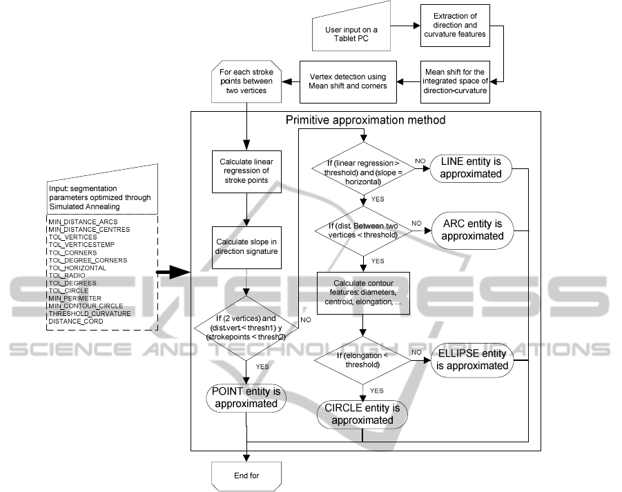
Figure 1: Flow chart of the segmentation algorithm (segmentation parameters listed in Table 1).

optimization algorithms to computer vision

problems: Taylor and Wolf (2004) applied an

optimization approach to improve the settings of

their text detection algorithm in images and video

sequences. Mbogho and Scarlatos (2007) used a

genetic algorithm to tune the colour thresholds to

minimize the effects of lighting variations on the

recognition of colored visual tags. Gelasca,

Salvador and Ebrahimi (2003) proposed a

framework for an intuitive tuning of parameters in

image and video segmentation algorithms. Other

applications to processes related to computer vision

have been developed by Mukerjee et al. (1997),

Davis et al. (2008), or Iakovidis et al. (2007).

The article is organized in the following way:

first the segmentation process is explained

(including the sketch correction, the vertices

detection procedure and the primitive approximation

method), secondly the implementation of the

optimization process by means of the simulated

annealing algorithm is detailed, and finally,

experimental work and results are given.

2 THE SEGMENTATION

ALGORITHM

Our application SegSGeo (Segmenting Sketched

Geometry) analyzes a stroke when a pen up event is

encountered, and fits the sketch into an outlined

sketch (poly-line). Its structure is shown in figure 1

and the procedure consists of five steps:

1. Direction and curvature signatures of the

stroke are calculated.

2. The mean shift (smoothing technique)

procedure is applied to the two previous

signatures (Yu, 2003).

3. Changes in direction of strokes are detected,

and vertices are fixed using peaks in

smoothed curvature signature.

GRAPP 2011 - International Conference on Computer Graphics Theory and Applications

322

4. A refinement of vertices is carried out when

their path length is less than a desired

threshold fixed empirically.

5. Finally, the type of each entity between a pair

of vertices is decided by means of a primitive

approximation method. Supported entities are

lines, arcs, circles and ellipses, and its type is

decided by looking into the direction

signature before Mean shift is applied, and

analyzing the points corresponding to that

piece of the stroke.

2.1 Extraction of Direction

and Curvature Signatures

The stroke is composed by a set of coordinates (x,y)

in an interval of pen-down and pen-up events. In

such a stroke, there are two visual features which

can guide recognition: direction and curvature. The

direction gives the angles between two consecutive

pairs of coordinates in the range [-π,π]. The

curvature gives the arctangent of the direction

between two consecutive points, to inform on how

opened or closed such piece of the stroke is.

2.2 Finding Vertices

Mean shift procedure (1) has been used to smooth

the collected stroke, since it has proven to give good

results in analyzing clusters in feature space, and in

eliminating noise (Yu, 2003).

,...2,1,

⎟

⎠

⎞

⎜

⎝

⎛

−

⎟

⎠

⎞

⎜

⎝

⎛

−

∑

(1)

In order to apply this procedure to the two-

dimensional direction-curvature joint space, we will

consider x

, i=1,2…n (where n is the number of

points in the direction-curvature joint space) as the

input vector of the mean shift procedure, that is, the

joint space d

and c

; and z

as the output vector of

smoothed discrete values of direction and curvature,

that is, the new direction and curvature signatures

after smoothing. The term k’ is the derivative of the

profile of Gaussian kernel k(x) = exp(−x / 2), and the

term h is the “bandwidth”, that is, the smoothing

parameter, which has been adjusted to h

and h

depending on direction and curvature respectively.

The smoothed curvature signature guides us to

find vertices in the stroke when seeking for local

maxima values, that is, where curvature changes

considerably (peaks in curvature signature figure

2c). The vertices seek routine finishes merging two

consecutive vertices when the path length between

them is lower than a threshold.

In the example of figure 2, six vertices are found,

and the first entity is approximated to an arc (arc

through 3 points: initial, final and middle of the first

section of the stroke) and the rest of entities to lines.

This has been achieved looking into both, the

original direction signature before mean shift

procedure between each two consecutive vertices,

and the correlation with the linear regression of the

stroke points of each entity, what is done by means

of the primitive approximation method.

Freehand sketch composed of 1

arc and 4 lines (in this order) A)

Direction signature

Curvature signature B)

Result of segmentation

process D)

Direction signature after

smoothing

Curvature signature after

smoothing C)

Figure 2: Example of a sketched figure.

2.3 Primitive Approximation Method

and Segmentation Parameters

The original direction signature and the correlation

of the stroke points from their linear regression are

used to identify the primitive entities composing a

stroke. If the features of the corresponding stroke

points are analyzed and the direction signature is

found to be horizontal, then that section of the stroke

is approximated to a line; otherwise it can be

approximated to an arc, circle or ellipse (see Figure

3). To approximate the section to an arc entity, the

direction signature must be inclined and the vertex

ends V

and V

separated, thus the section is fitted to

an arc by three points V

, V

and s. If the vertices are

close, the section is approximated to a circle or

ellipse depending on the elongation (quotient

between major R and minor r radius).

The segmentation process is controlled by 14

parameters, listed in Table 1. For each parameter a

range of values from previous observations has been

established (range column).

AUTOMATED TUNING OF PARAMETERS FOR THE SEGMENTATION OF FREEHAND SKETCHES

323

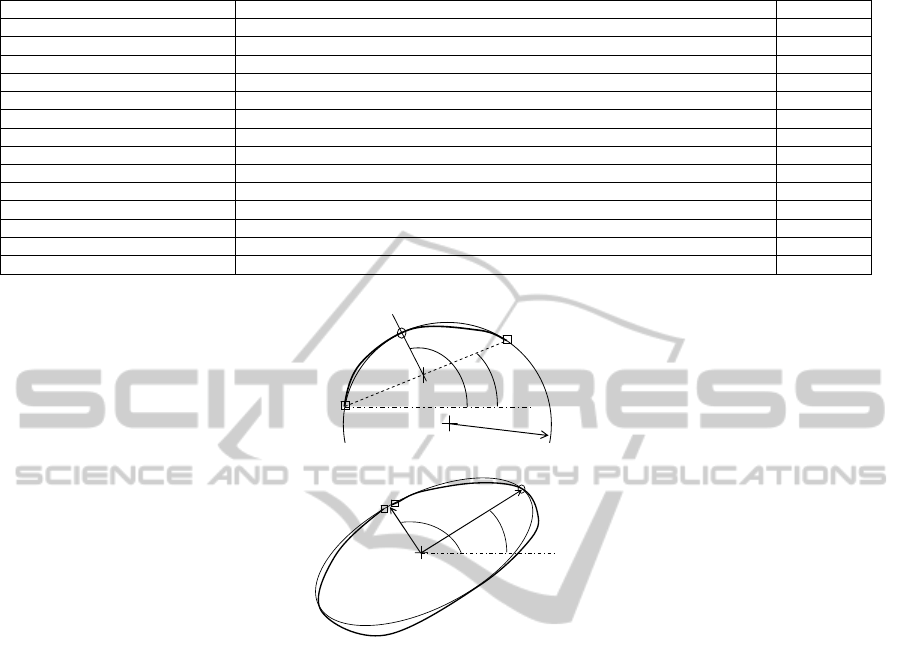
Table 1: Parameters of the segmentation and its initial range.

Parameter Description Range

MIN_DISTANCE_ARCS Distance between the two ends of an arc [0,50]

MIN_DISTANCE_CENTRES* Distance between the centers of two consecutive arcs [0,100]

TOL_VERTICES Tolerance for the distance between two consecutive vertices [0,30]

TOL_VERTICESTEMP Involved in the seek for local maximums and minimums [1,30]

TOL_CORNERS Distance from a point to both sides to calculate the angle of a corner [1,20]

TOL_DEGREE_CORNERS Threshold to considerate a corner as a vertex [1,60]

TOL_HORIZONTAL Tolerance for a horizontal slope [0,0.05]

TOL_RADIO* Tolerance for large values of radio [200,600]

TOL_DEGREES* Tolerance for the orientation of two consecutive lines [0º,30º]

TOL_CIRCLE Tolerance for the quotient of diameters to distinguish a circle from ellipse [0.3,0.8]

MIN_PERIMETER Minimum length for a line or arc [2,10]

MIN_CONTOUR_CIRCLE Minimum contour for circle or ellipse [30,200]

THRESHOLD_CURVATURE Tolerance for vertices in order to consider the stroke a circle or ellipse [0.1,0.5]

DISTANCE_CORD Arc length to help the decision of an arc or a line [20,300]

* Refinement parameters.

Mid

oint

Intersection

oint

α+π/2

a) Fitting a stretch of sketch to an arc.

α+π/2

b) Fitting a stretch of sketch to a circle/ellipse.

Figure 3: Parameters calculated for arcs/circles/ellipses entities.

3 TUNING OF SEGMENTATION

PARAMETERS

The steps for tuning the parameters of the

segmentation process consist of four main parts:

1. Definition of the initial range of values for

each segmentation parameter based on

previous experience.

2. Automatic tuning of parameters inside their

initial range using a simulated annealing

algorithm.

3. Definition of the definitive range of values

for each segmentation parameter, analyzing

the behaviour of each parameter when the

rest of parameters are fixed to their optimal

values.

4. Automatic tuning of parameters inside their

definitive range using a simulated annealing

algorithm.

The quality of the obtained segmentation is

evaluated by means of a cost function (2) that

returns a real value (cost) from a set of n

segmentation parameters P = {p

, p

, ... p

ℜ

→Pc :

(2)

The cost value for a set of parameters is defined

as the ratio of bad segmented shapes using this set of

parameters. A library of sketched figures and their

correct segmentation has been developed in order to

implement the cost function (examples at Figure 4).

The correct or ideal segmentation has been

previously defined by consensus by the research

team of this work. The criteria applied to define a

well segmented shape are based on an all-or-nothing

accuracy, that is, a shape is well segmented if:

 The number of vertices must match the

ideal segmentation.

GRAPP 2011 - International Conference on Computer Graphics Theory and Applications

324

 The type of fitted primitives connecting the

vertices must match the intended primitives

of ideal segmentation.

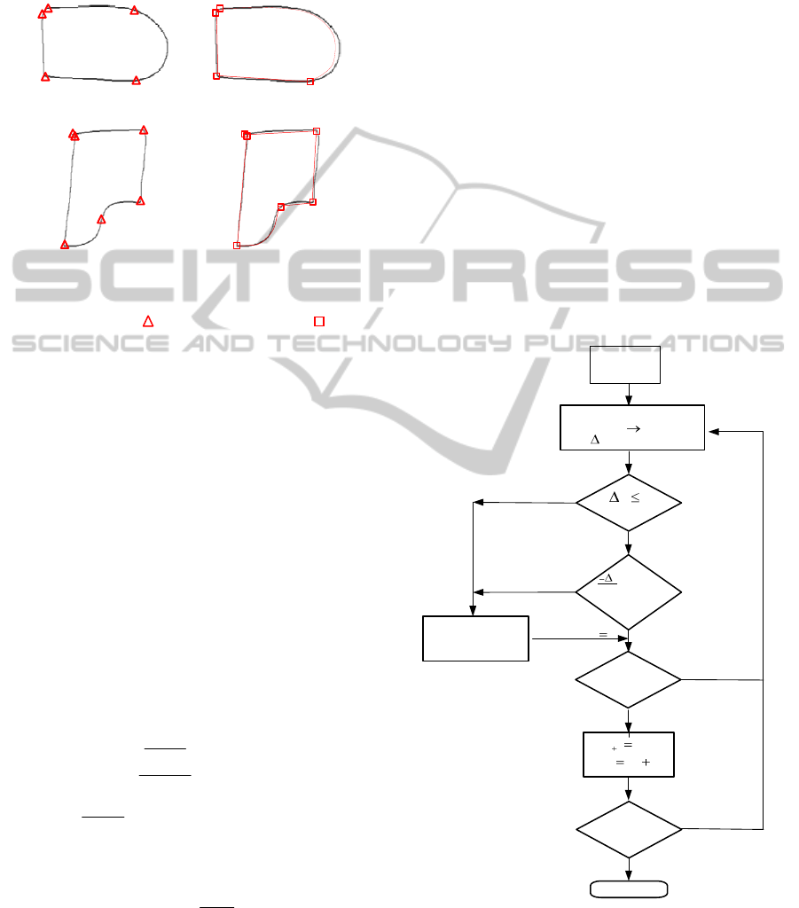
Sketched shape and correct

segmentation

Result of

segmentation

Primitives=1 line, 1 arc, 2 lines



Primitives=1 arc, 2

lines

Primitives=2 lines, 2 arcs, 1

line



Primitives=3 lines, 1

arc, 2 lines

Figure 4: Examples of missegmentations. (Intended

segmentation vertex ( ), recognized vertex ( ) and

recognized primitive in red color).

3.1 Tuning of Parameters using a

Simulated Annealing Algorithm

The next step carried out to determine the optimal

range of the segmentation parameters is

implemented by a simulated annealing algorithm

(Kirkpatrick, Gelatt and Vecchi, 1983). The SA

algorithm is shown in figure 5 and described below.

The parameters involved in the SA algorithm can be

classified as generic or specific.

The “generic parameters” or "annealing

schedule" control the operation of the algorithm.

They are:

 Initial Temperature: initial value of temperature

at the beginning of the SA process. It is

calculated using the following expression

(Kouvelis et al., 1992):

()

−

(3)

where

()

ΔC

is the mean value of the cost

increment associated to those displacements

with an increment in the cost function. In our

particular case, the tests performed show that

for 100 displacements,

()

5.1≈Δ

. Where χ

the expected initial coefficient of acceptance (χ

is the rate of accepted displacements with

respect to the total number of attempts). Using

a typical value of this coefficient in the

literature (χ

=0.75), the resulting value for

initial temperature is T

≈5.

 Cooling Schedule: indicates how temperature

varies from two different steps. The more

common form consists of a potential cooling

(faster with high temperatures):

TkT

⋅

(4)

where m is the current temperature step, and k

is the cooling coefficient. A rapid cooling

(small values of k) causes a quick fall in the

cost, but if it is too fast, the SA may exit

without reaching good solutions. Moreover, a

slow cooling down makes the cost function to

have ups and downs (high cost displacement

are allowed) but increases the number of

iterations (the time required) and the

probability of finding the optimal solution. A

value of 0.5 has shown a good compromise

with respect to cost and speed.

END

Frozen

system

Change

temperature

> random(0,1)

Accept new solution

= n

+ 1

Generating new solution

m = n

= n = 0

Solution j-1 Solution j

c= c(P

)-c(P

j-1

)

yes

Initialization

Calculate To

n = n + 1

TkT

mm1

= n = 0

Figure 5: SA algorithm.

 Balance Criterion (change temperature): it

decides when the temperature must go

AUTOMATED TUNING OF PARAMETERS FOR THE SEGMENTATION OF FREEHAND SKETCHES

325

downhill to the next step using this logical

condition:

(

)

()

max

nnORnn

(5)

Where:

o n

is the number of successful displacements

in the present temperature step.

o n

max

is the maximum number of successful

displacements in a temperature step. Usually

this number is determined according to the

size of the space of solutions. In this problem,

the used value is the number of parameters to

optimize, in this case with 14 parameters,

max

=14.

o n is the number of attempted displacements in

the present temperature step.

o n

max

is the maximum number of attempted

displacements in a temperature step, and

usually is proportional to the n

max

value. In

the current context, n

max

= 2· n

max

, so n

max

=28.

 Freezing Criterion: it is the stop criterion that

terminates the SA process:

()

(

)

max

min

mmOR ><

χχ

(6)

The freezing condition can be accomplished

when the temperature has experimented a

specific number of downhill moves (m

max

), or

when the coefficient of acceptance is very low

(χ = n

/ n), where:

min

is the minimum coefficient of

acceptance, in this case 1% is the selected

value.

o m

max

is the maximum allowed number of

temperature steps, in this case the selected

value is 50.

The specific parameters of the SA in the context

of our problem are:

 The Space of Solutions P, that in this case

corresponds to the 14 parameters used for

segmentation (see table 1):

P = {p

, p

, ... p

}

(7)

 A displacement mechanism for choosing a

solution nearby the current one. For each

parameter pi to optimize in the iteration j, its

value is obtained from its previous value (from

the iteration j-1) as follows:

ijijiij

ξδ

⋅+=

− )1(

(8)

Where p

∈

min

, p

max

], δ

=α·(p

max

- p

min

and α is the maximum displacement ratio (α =

0.1 provided a good performance in the current

problem).

is a random number in the range

[−1,1], obtained for each parameter in each

iteration.

 The cost function

ℜ→Pc :

that gives a value

that must be minimized. For a training set of nt

sketched figures this function is defined as:

c = n

/ n

(9)

Where n

is the number of mistakes

corresponding to those bad segmented shapes

applying the criterion defined at the beginning

of section 3.

The best solution obtained during the

optimization process is stored, in order to avoid

situations where the final solution does not

correspond to the optimal one.

100

0 100 200 300 400 500

Figure 6: Cost and temperature evolution in a SA process.

3.2 Individual Parameter Adjustment

After the first simulated annealing step, in order to

establish the definitive range for a specific parameter

we have fixed the rest of the parameters to their

optimal value (obtained from the previous simulated

annealing step), and the cost is obtained with the

parameter p

ranged in its whole initial range (and

expanded if it is necessary). The definitive range is

fixed centring it in the optimal value obtained from

the process and expanded or compressed if it is

necessary.

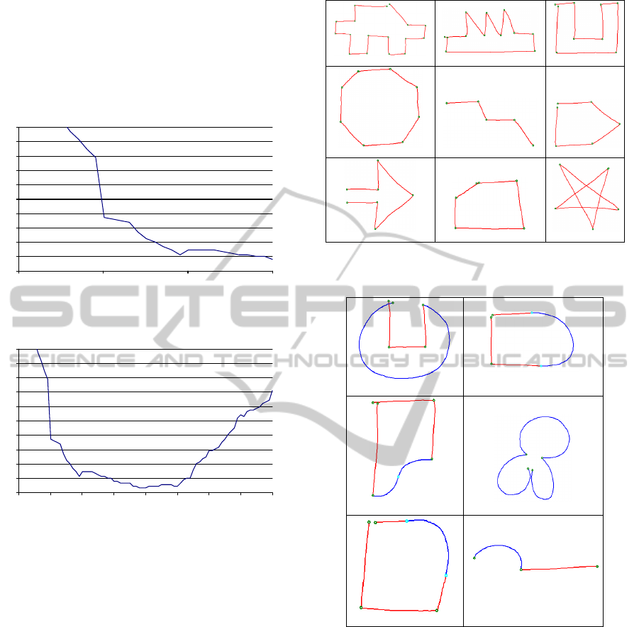
Figure 7 shows the initial or default range for the

segmentation parameter TOL_VERTICES fixed

from expertise. As notice, the value of this

parameter for the minor cost function is beyond the

right value 30, so best results in segmentation are

never reached. Figure 8 shows the corrected range

for this parameter. Now, the optimal value is

Best solution

Local minimum

Cost / Temperature

Iterations

GRAPP 2011 - International Conference on Computer Graphics Theory and Applications

326

centered in the range so better results in

segmentation can be achieved.

So, the value of the parameter for the lowest

function cost has been centered in a range, and its

width has been fixed in order to avoid the function

cost increase more than a percentage. This width is

variable for each parameter.

0102030

Initialrange:[0,30]

Figure 7: Initial range for parameter TOL_VERTICES.

0 1020304050607080

Definitiverange:[0,80]

Figure 8: Definitive range for parameter TOL_VERTICES

after the correction process.

When all the ranges have been adjusted, the

second simulated annealing step provides the final

segmentation parameter values.

4 EXPERIMENTAL WORK

The segmentation process has been applied to a set

of 177 samples of 20 different sketched figures

(including circle and ellipse) collected from 3 users

and stored in a DB. Each user drew 3 samples of

each figure, and 3 figures with poor quality were

discarded.

Figures 9 and 10 show some examples of

sketched figures segmented using the parameters

optimized with the SA algorithm.

Sample01

Sample02 Sample03

Sample04

Sample05 Sample06

Sample09

Sample10 Sample11

Figure 9: Examples of sketched figures used in the tests

including only lines.

Sample12

Sample13

Sample17

Sample18

Sample20

Sample14

Figure 10: Examples of sketched figures used in the tests

including lines (in red) and arcs (in blue).

The segmentation process has been carried out

with a different set of segmentation parameters for

each SA iteration. And the SA process has been

made up with different ranges for segmentation

parameters and different values for SA parameters as

described in section 3.

5 CONCLUSIONS

From results obtained, we can state that the

optimization process improves significantly the

AUTOMATED TUNING OF PARAMETERS FOR THE SEGMENTATION OF FREEHAND SKETCHES

327

results of the segmentation, demonstrating that, in

general, the recognition process can benefit much if

optimization techniques are applied to its parameters

tuning them for their optimal values. The results

improved in more than 10% respect those obtained

with previous parameters fixed empirically from

observation. The segmentation approach SegSGeo

with the optimization process obtained a success of a

92% of well segmented figures (all-or-nothing-

accuracy), which increases to 97% if we consider

isolated entities instead of complete figures.

With respect to the optimization technique, tests

with different SA parameters show a very stable

behavior of SA algorithm, so it can find good

solutions though the SA parameters vary within a

fairly wide range. The most critical parameter is the

displacement mechanism, that is, the maximum

displacement ratio α: it must be high enough to get

out from local minimum, but not too high to avoid

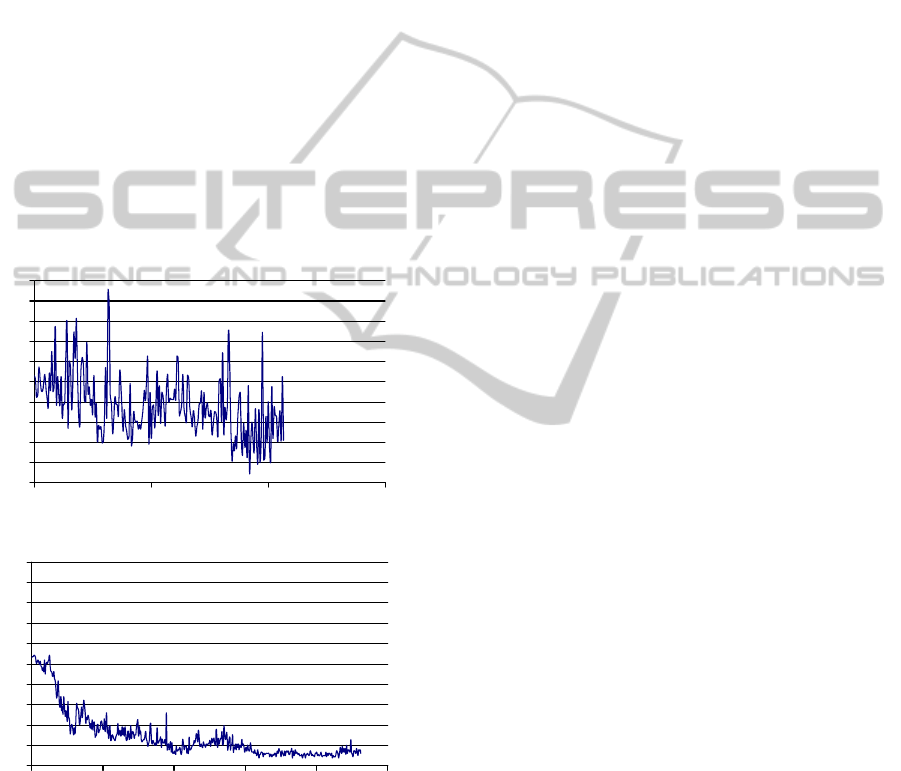
jumping haphazardly (see figure 11).

100

0 100 200 300

100

0 100 200 300 400 500

Figure 11: Cost evolution in two different SA processes

(above: α=0.4) (below: α=0.1).

The following parameters in order of importance

are those that control the cooling scheme: the initial

temperature T

and cooling coefficient k. The

probability of finding an optimal solution increases

when more tests are performed with a slow cooling

(higher T

, or k closest to 1), but increasing the time

too. Good solutions can be found with a set of SA

process with a fast cooling scheme or with a single

SA process with a slow cooling scheme.

Tests show that classical values for balance and

freezing criterions (dependent on the number of

parameters to optimize) are appropriate. On the one

hand, changes in balance criterion have a similar

effect that changes in cooling scheme, on the other

hand, changes on freezing criterion do not

significantly affect the SA time or result.

REFERENCES

Azar, S., Couvreury, L., Delfosse, V., Jaspartz, B. and

Boulanger, C. (2006). An agent-based multimodal

interface for sketch interpretation. In Proceedings of

International Workshop on Multimedia Signal

Processing (MMSP-06), 488 - 492.

Casella, G., Deufemia, V., Mascardi, V., Costagliola, G.

and Martelli, M. (2008). An agent-based framework

for sketched symbol interpretation. Journal of Visual

Languages and Computing, 19, 225–257.

Davis, R. C., Colwell, B. and Landay, J. A. (2008). K-

Sketch: A ‘Kinetic’ Sketch Pad for Novice Animators.

Proceedings of the twenty-sixth annual SIGCHI

conference on Human factors in computing systems.

Aesthetics, Awareness, and Sketching, 413-422.

Fernández-Pacheco, D. G., Aleixos, N., Conesa, J. and

Contero, M. (2009). Natural interface for sketch

recognition. Advances in Intelligent and Soft

Computing, 55, 510-519.

Fernández-Pacheco, D. G., Conesa, J., Aleixos, N.,

Company, P. and Contero, M. (2009). An agent-based

paradigm for free-hand sketch recognition. Lecture

Notes in Artificial Intelligence, 5883, 345-354.

Flasinski, M., Jurek, J. and Myslinski, S. (2009). Multi-

agent System for Recognition of Hand Postures.

Lecture Notes in Computer Science, 5545, 815-824.

Gelasca, E. D., Salvador, E. and Ebrahimi, T. (2003).

Intuitive strategy for parameter setting in video

segmentation. Visual communications and image

processing, SPIE proceedings series, 5150 (3), 998-

1008.

Iakovidis, D. K., Savelonas, M. A., Karkanis, S. A. and

Maroulis, D. E. (2007). A genetically optimized level

set approach to segmentation of thyroid ultrasound

images. Applied Intelligence, 27 (3), 193-203.

Juchmes, R., Leclercq P. and Azar, S. (2005). A freehand-

sketch environment for architectural design supported

by a multi-agent system. Computers & Graphics, 29

(6), 905–915.

Kirkpatrick, S., Gelatt, C. D. and Vecchi, M. P. (1983).

Optimization by Simulated Annealing. Science, 220

(4598), 671-680.

Kouvelis, P. and Chiang, W. C. (1992). A simulated

annealing procedure for single row layout problems in

Cost

Iterations

Cost

Iterations

GRAPP 2011 - International Conference on Computer Graphics Theory and Applications

328

flexible manufacturing systems, International Journal

of Production Research, 30 (4), 717-732.

Mbogho, A. J. & Scarlatos, L. L. (2007). Genetic

parameter tuning for reliable segmentation of colored

visual tags. In Proceedings of the 9th Annual

Conference on Genetic and Evolutionary

Computation, ACM, 1525-1525.

Mukerjee, A., Agrawal, R. B., Tiwari, N. and Hasan, N.

(1997). Qualitative sketch optimization. Artificial

intelligence for engineering design, analysis and

manufacturing, 11 (4), 311-323.

Taylor, G. W. & Wolf, C. (2004). Reinforcement Learning

for Parameter Control of Text Detection in Images and

Video Sequences. In Proc. of the IEEE International

Conference on Information & Communication

Technologies.

Varley, P. & Company, P. (2008). Automated sketching

and engineering culture. In Proceedings of VL/HCC

Workshop Sketch Tools for Diagramming, 83-92.

Yu, B. (2003). Recognition of freehand sketches using

mean shift. In Proceedings of IUI, 204–210.

AUTOMATED TUNING OF PARAMETERS FOR THE SEGMENTATION OF FREEHAND SKETCHES

329