
PARTIAL UPDATE CONJUGATE GRADIENT ALGORITHMS
FOR ADAPTIVE FILTERING
Bei Xie and Tamal Bose
Wireless @ Virginia Tech, Bradley Department of Electrical and Computer Engineering
Virginia Polytechnic Institute and State University, Blacksburg, VA 24061, U.S.A.
Keywords:
Conjugate gradient adaptive filter, Partial update, Recursive algorithms.
Abstract:
In practice, computational complexity is an important consideration of an adaptive signal processing system.
A well-known approach to controlling computational complexity is applying partial update (PU) adaptive
filters. In this paper, a partial update conjugate gradient (CG) algorithm is employed. Theoretical analyses of
mean and mean-square performance are presented. The simulation results of different PU CG algorithms are
shown. The performance of PU CG algorithms are also compared with PU recursive least squares (RLS) and
PU Euclidean direction search (EDS) algorithms.
1 INTRODUCTION
Adaptive filters play an important role in fields re-
lated to digital signal processing, such as system iden-
tification, noise cancellation, and channel equaliza-
tion. In the real world, the computational complex-
ity of an adaptive filter is an important considera-
tion for applications which need long filters. Usually
least squares algorithms, such as RLS, EDS (Bose,
2004), and CG, have higher computational complex-
ity and give better convergence performance than the
steepest-descent algorithms. Therefore, a tradeoff
must be made between computational complexity and
performance. One option is to use partial update tech-
niques (Do˘ganc¸ay, 2008) to reduce the computational
complexity. The partial update adaptivefilter only up-
dates part of the coefficient vector instead of updating
the entire vector. The theoretical results on the full-
update case may not apply to the partial update case.
Therefore, performance analysis of the partial update
adaptive filter is very meaningful. In the literature,
partial update methods have been applied to several
adaptive filters, such as Least Mean Square (LMS),
Normalized Least Mean Square (NLMS), RLS, EDS,
Affine Projection (AP), Normalized Constant Mod-
ulus Algorithm (NCMA), etc. Most analyses are
based on LMS and its variants (Douglas, 1995), (Dou-
glas, 1997), (Godavarti and Hero III, 2005), (Mayyas,
2005), (Khong and Naylor, 2007), (Wu and Doroslo-
vacki, 2007), (Do˘ganc¸ay, 2008). There are some
analyses for least squares algorithms. In (Naylor
and Khong, 2004), the mean and mean-square per-
formance of the MMax RLS has been analyzed for
white inputs. In (Khong and Naylor, 2007), the track-
ing performance has been analyzed for MMax RLS.
In (Xie and Bose, 2010), the mean and mean-square
performance of PU EDS are studied.
In this paper, partial update techniques are applied
to the CG algorithm. CG solves the same cost func-
tion as the RLS algorithm. It has a fast convergence
rate and can achieve the same mean-square perfor-
mance as RLS at steady state. It has lower compu-
tational complexity when compared with the RLS al-
gorithm. The EDS algorithm is a simplified CG algo-
rithm, and it has lower computational complexity than
the CG algorithm. The basic partial update methods
such as periodic PU, sequential PU, stochastic PU,
and MMax update method, are applied to the CG al-
gorithm. The mean and mean-square performance of
different PU CG are analyzed, and compared with the
full-update CG algorithm. The goal of this paper is
to find one or more PU CG algorithms which can re-
duce the computational complexity while maintaining
good performance. In Section 2, different PU CG al-
gorithms are developed. Theoretical mean and mean-
square analyses of PU CG for white input are given in
Section 3. In Section 4, computer simulation results
are shown. The performance of different PU CG al-
gorithms are compared. The performance of PU CG,
PU RLS, and PU EDS are also compared.
317
Xie B. and Bose T. (2011).
PARTIAL UPDATE CONJUGATE GRADIENT ALGORITHMS FOR ADAPTIVE FILTERING.
In Proceedings of the 1st International Conference on Pervasive and Embedded Computing and Communication Systems, pages 317-323
DOI: 10.5220/0003364103170323
Copyright
c
SciTePress

2 CG AND PARTIAL UPDATE CG
The basic adaptive filter system model can be written
as:
d(n) = x
T
(n)w
∗
+ v(n), (1)
where d(n) is the desired signal, x(n) = [x(n),x(n −
1),..., x(n − N + 1)]
T
is the input data vector of the
unknown system, w
∗
(n) = [w
∗
1
,w
∗
2
,...,w
∗
N
]
T
is the im-
pulse response vector of the unknown system, and
v(n) is zero-mean white noise, which is independent
of any other signal.
Let w be the coefficient vector of an adaptive filter.
The estimated signal y(n) is defined as
y(n) = x
T
(n)w(n− 1), (2)
and the output signal error is defined as
e(n) = d(n) − x
T
(n)w(n− 1). (3)
Since the CG algorithm with reset method needs
higher computational complexity than the non-reset
method, we consider only the CG with non-reset
Polak-Ribi`ere (PR) method. The CG with PR method
(Chang and Willson, 2000) is summarized as follows:
Initial conditions:
w(0) = 0, R(n) = 0, p(1) = g(0).
e(n) = d(n) − x
T
(n)w(n− 1), (4)
R(n) = λR(n− 1) + x(n)x
T
(n), (5)
α(n) = η
p
T
(n)g(n− 1)
p
T
(n)R(n)p(n)
, (6)
w(n) = w(n− 1) + α(n)p(n), (7)
g(n) = λg(n− 1) − α(n)R(n)p(n)
+x(n)e(n), (8)
β(n) =
(g(n) − g(n− 1))
T
g(n)
g
T
(n− 1)g(n− 1)
, (9)
p(n+ 1) = g(n) + β(n)p(n), (10)
where R is the time-average correlation matrix of x,
p is the search direction, and g is the residue vector
which is also equal to b(n)−R(n)w(n), where b(n) =
λb(n−1)+x(n)d(n) is the estimated crosscorrelation
of x and d. The choice of g(0) can be d(1)x(1) or
satisfies g
T
(0)g(0) = 1. λ is the forgetting factor and
the constant parameter η satisfies λ− 0.5 ≤ η ≤ λ.
The partial update method aims to reduce the com-
putational cost of the adaptive filters. Instead of up-
dating all the N × 1 coefficients, it usually only up-
dates M × 1 coefficients, where M < N. Basic partial
update methods include periodic PU, sequential PU,
stochastic PU, and MMax update method, etc. These
methods will be applied to the CG algorithm. For the
CG algorithm, the calculation of R needs high compu-
tational cost. To reduce the computational complex-
ity, the subselected tap-input vector ˆx = I
M
x is used.
The partial update CG algorithm is summarized as
follows:
e(n) = d(n) − x
T
(n)w(n− 1), (11)
ˆ
R(n) = λ
ˆ
R(n− 1) +
ˆ
x(n)
ˆ
x
T
(n), (12)
α(n) = η
p
T
(n)g(n− 1)
p
T
(n)
ˆ
R(n)p(n)
, (13)
w(n) = w(n− 1) + α(n)p(n), (14)
g(n) = λg(n− 1) − α(n)
ˆ
R(n)p(n)
+ˆx(n)e(n), (15)
β(n) =
(g(n) − g(n− 1))
T
g(n)
g
T
(n− 1)g(n− 1)
, (16)
p(n+ 1) = g(n) + β(n)p(n), (17)
where
ˆ
x = I
M
x, (18)
and
I
M
(n) =
i
1
(n) 0 .. . 0
0 i
2
(n)
.
.
.
.
.
.
.
.
.
.
.
.
.
.
.
0
0 . .. 0 i
N
(n)
, (19)
N
∑
k=1
i
k
(n) = M, i
k
(n) ∈ {0,1}, (20)
For each iteration, only M elements of the input vec-
tor are used to update the weights. Note, the calcu-
lation of output signal error still uses the the whole
input vector, not the subselected input vector. The
total number of multiplications of full-update CG is
3N
2
+ 10N + 3 per sample. The total number of
multiplications of partial-update CG is reduced to
2N
2
+ M
2
+ 9N + M + 3 per sample. The computa-
tional complexity of different PU methods is not con-
sidered here.
2.1 Periodic Partial Update CG
The periodic partial update method (Do˘ganc¸ay, 2008)
only updates the coefficients at every S
th
iteration and
copies the coefficients at the other iterations. The pe-
riodic PU CG updates the weights at every S
th
itera-
tion. The update equation for periodic PU CG can be
written as:
w(nS) = w((n− 1)S) + α(nS)p(nS), (21)
where S =
N
M
, which is the ceiling of
N
M
. Since
the periodic PU CG still uses the whole input vec-
tor, the steady-state performance will be the same as
PECCS 2011 - International Conference on Pervasive and Embedded Computing and Communication Systems
318

the full-update CG. However, the convergence rate of
the periodic PU CG will be S times slower than the
full-update CG.
2.2 Sequential Partial Update CG
The sequential partial update method (Do˘ganc¸ay,
2008) designs i
k
(n) as:
i
k
(n) =
1 if k ∈ K
n mod S+1
0 otherwise
, (22)
where K
1
= {1,2,...,M}, K
2
= {M + 1,M +
2,. ..,2M}, ... , K
S
= {(S − 1)M + 1, (S − 1)M +
2,. ..,N}.
2.3 Stochastic Partial Update CG
The stochastic partial update CG chooses input vector
subsets randomly. The i
k
(n) becomes
i
k
(n) =
1 if k ∈ K
m(n)
0 otherwise
, (23)
where m(n) is a random process with probability mass
function (Do˘ganc¸ay, 2008):
Pr{m(n) = i} = p
i
, i = 1, ...,S,
S
∑
i=1
p
i
= 1. (24)
Usually a uniformly distributed random process will
be applied. Therefore, for each iteration, M of N input
elements will be chosen with probability p
i
= 1/S.
2.4 MMax CG
The MMax CG selects the input vector according to
the first M max elements of the input x. The condition
of i
k
(n) (Do˘ganc¸ay, 2008) becomes
i
k
(n)=
1 if |x
k
(n)| ∈ max
1≤l≤N
{|x
l
(n)|,M}
0 otherwise
. (25)
The sorting of the input x increases the computa-
tional complexity. It can be achieved efficiently us-
ing the SORTLINE or Short-sort methods (Chang
and Willson, 2000). The SORTLINE method needs
2+ 2log
2
N multiplications.
3 PERFORMANCE ANALYSIS OF
PARTIAL UPDATE CG
The normal equation of the partial update CG algo-
rithm can be represented as:
X
T
M
(n)Λ(n)X(n)w(n) = X
T
M
(n)Λ(n)d(n), (26)
where d(n) = [d(n),d(n− 1),...,d(1)]
T
,
X
M
(n) =
ˆ
x
T
M
(n)
ˆ
x
T
M
(n− 1)
.
.
.
ˆ
x
T
M
(1)
, (27)
and
Λ(n) =
1 0 .. . 0
0 λ
.
.
.
.
.
.
.
.
.
.
.
.
.
.
.
0
0 . .. 0 λ
n
. (28)
Therefore, the residue vector g can also be written as
g =
ˆ
b(n) −
e
R(n)w(n), (29)
where
e
R(n) = λ
e
R(n− 1) +
ˆ
x(n)x
T
(n), (30)
ˆ
b(n) = λ
ˆ
b(n− 1) + ˆx(n)d(n). (31)
To simplify the analysis, we assume that the in-
put signal is wide-sense stationary and ergodic, and
α(n), β(n),
e
R(n), and w(n) are uncorrelated to each
other (Chang and Willson, 2000). Apply the ex-
pectation operator to (14), (15), and (17). De-
fine E{α(n)} =
¯
α, E{β(n)} =
¯
β, E{
ˆ
b(n)} =
ˆ
b, and
E{
e
R(n)} =
e
R. The system can be viewed as lin-
ear and time invariant at steady state. Therefore, the
Z -transform can be applied to the system. Define
W(z) = Z {E{w(n)}}, G(z) = Z {E{g(n)}}, and
P(z) = Z {E{p(n)}}. Equations (14), (15), and (17)
become
W(z) = W(z)z
−1
+
¯
αP(z), (32)
G(z) =
ˆ
bz
z− 1
−
e
RW(z), (33)
zP(z) = G(z) +
¯
βP(z). (34)
Therefore,
W(z) = [(z− 1)(z− β)I+ α
e
Rz]
−1
α
ˆ
bz
2
z− 1
. (35)
Since the system is causal and n ≥ 0, the Z -transform
is one-sided and W(z) = W
+
(z). At steady state, the
mean of weights converge to
lim
n→∞
E{w(n)} = lim
z→1
W
+
(z)
=
e
R
−1
ˆ
b. (36)
For the causal system to be stable, all the poles must
be inside the unit circle. Therefore, the conditions
for the stability are |
¯
β| < 1 and 0 ≤
¯
α ≤
2
¯
β+2
λ
max
, where
PARTIAL UPDATE CONJUGATE GRADIENT ALGORITHMS FOR ADAPTIVE FILTERING
319
λ
max
is the maximal eigenvalue of
e
R. For the sequen-
tial and stochastic methods, the partial update correla-
tion matrix
ˆ
R may become ill-conditioned, especially
when M becomes smaller, and the algorithm may suf-
fer convergence difficulty. More sophisticated analy-
sis will be provided in a future paper.
Since the input noise v(n) is assumed to be zero
mean white noise and independent of the input sig-
nal x(n), the MSE equation of the PU CG algorithm
becomes
E{|e(n)|
2
} = σ
2
v
+ tr(RE{ε(n)ε
T
(n)}), (37)
where σ
2
v
= E{v
2
(n)} is the variance of the input
noise, and ε(n) = w
∗
− w(n) is the weight error vec-
tor. To simplify the analysis, it is also assumed that
the weight error ε(n) is independent of the input sig-
nal x(n) at steady state, and the input signal is white.
At steady state,
w(n) ≈
e
R
−1
(n)
ˆ
b(n). (38)
Using (30), (31), and (1), w(n) can be written as
w(n) ≈ w
∗
+
e
R
−1
(n)
n
∑
i=1
λ
n−i
ˆ
x(i)v(i). (39)
Define the weight error correlation matrix as
K(n) = E{ ε(n)ε
T
(n)}
= E{(w
∗
− w(n))(w
∗
− w(n))
T
}. (40)
Substituting (39) into (40) and applying the assump-
tions, we get
K(n) ≈ E{
e
R
−1
(n)
n
∑
i=1
n
∑
j=1
λ
n−i
λ
n− j
ˆ
x(i)
ˆ
x
T
( j)
e
R
−T
(n)}
E{v(i)v( j)}. (41)
Since the input noise is white,
E{v(i)v( j)} =
σ
2
v
for i = j
0 otherwise
. (42)
Therefore, K(n) becomes
K(n) ≈ σ
2
v
E{
e
R
−1
(n)
n
∑
i=1
λ
2(n−i)
ˆ
x(i)
ˆ
x
T
( j)
e
R
−T
(n)}
= σ
2
v
e
R
−1
b
b
R
e
R
−T
, (43)
where
b
b
R = E{
∑
n
i=1
λ
2(n−i)
ˆ
x(i)
ˆ
x
T
( j)}.
The MSE equation becomes
E{|e(n)|
2
} ≈ σ
2
v
+ σ
2
x
σ
2
v
tr(
e
R
−1
b
b
R
e
R
−T
), (44)
where tr(·) is the trace operator, and σ
2
x
= tr(R) is the
variance of the white input signal.
4 SIMULATIONS
4.1 Performance of Different PU CG
Algorithms
The convergence performance and mean-square per-
formance of different partial update CG algorithms
are compared in a system identification application.
The system identification model is shown in Figure
1 and is taken from (Zhang et al., 2006). The un-
known system (Mayyas, 2005) is a 16-order FIR filter
(N=16), with impulse response
w
∗
= [0.01, 0.02,−0.04,−0.08, 0.15,−0.3,0.45,0.6,
0.6,0.45,−0.3,0.15,−0.08, −0.04,0.02,0.01]
T
.
In our simulations, the length of the partial update fil-
ter is M=8. The variance of the input noise v(n) is
ε
min
= 0.0001. The initial weights are w = 0. The
parameters λ and η of CG are equal to 0.9 and 0.6,
respectively. The initial residue vector is set to be
g(0) = d(1)x(1). The results are obtained by aver-
aging 100 independent runs.
v(n)
x(n)d(n)ε(n)
_
Unknownsystem
Adaptivefilter
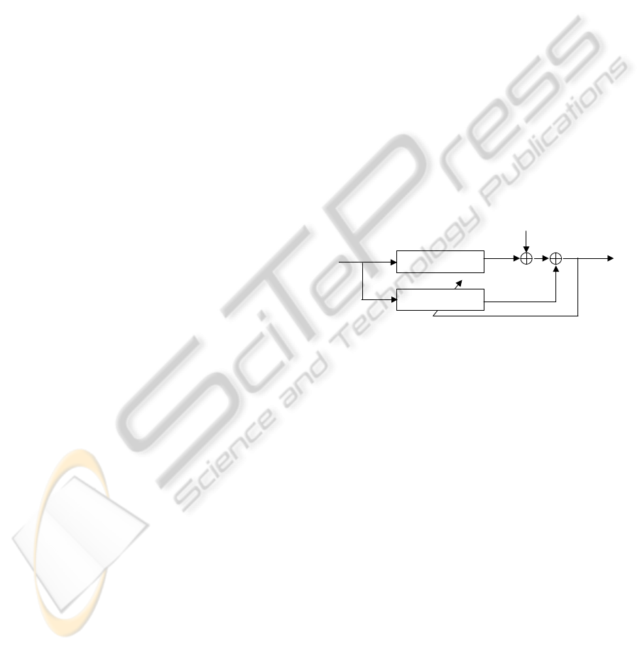
Figure 1: System identification model.
The correlated input of the system (Zhang et al.,
2006) has the following form
x(n) = 0.8x(n− 1) + ζ(n), (45)
where ζ(n) is zero-mean white Gaussian noise with
unit variance.
Figure 2 and Figure 3 show the mean-square error
(MSE) performance of the partial update CG for the
correlated input and white input, respectively. From
the figures, the steady-state MSE of the periodic PU
CG is the same as that of CG. The convergence rate of
the periodic PU CG algorithm is about N/M = 2 times
slower than the full-update CG algorithm. The MMax
CG converges a little faster than the periodic CG in
this case. The steady-state MSE of MMax CG is close
to the full-update CG. The sequential and stochastic
PU CG have higher MSE than the full-update CG at
steady state. Their convergence rates are slow.
Figure 4 shows the mean convergence of the
weights at steady state for MMax CG. The PU length
is 8, and the input signal is white. The theoretical
results are calculated from (36). We can see that
PECCS 2011 - International Conference on Pervasive and Embedded Computing and Communication Systems
320
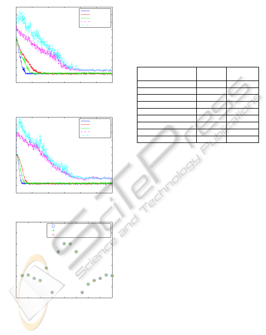
0 200 400 600 800 1000 1200
−50
−40
−30
−20
−10
0
10
20
30
40
50
samples
MSE(dB)
CG
Periodic CG
MMax CG
Sequential CG
Stochastic CG
Figure 2: Comparison of MSE of PU CG with correlated
input.
0 200 400 600 800 1000 1200
−50
−40
−30
−20
−10
0
10
20
30
40
50
samples
MSE(dB)
CG
Periodic CG
MMax CG
Sequential CG
Stochastic CG
Figure 3: Comparison of MSE of PU CG with white input.
0 2 4 6 8 10 12 14 16
−0.4
−0.2
0
0.2
0.4
0.6
0.8
1
index
weights
Optimal weights
Simulated weigths of MMax CG
Theoretical weigths of MMax CG
Figure 4: The mean convergence of the weights at steady
state for MMax CG.
the theoretical results match the simulated results.
The weights of MMax CG are close to the optimal
weights.
Table 1 shows the simulated MSE and theoretical
MSE of PU CG algorithms at steady state for white
input. The theoretical results are calculated from (44).
The partial-update lengths are M = 12, M = 8, and
M = 4. For sequential and stochastic PU CG, the al-
gorithms do not converge when PU length is 4. When
PU length reduces, the MSE of MMax CG increases
slowly, while the MSE of sequential and stochastic
increase rapidly.
Table 1: The simulated MSE and theoretical MSE of PU
CG algorithms.
Algorithms Simulated Theoretical
MSE (dB) MSE (dB)
MMax CG (M=12) -37.3869 -37.6732
MMax CG (M=8) -37.1362 -36.7467
MMax CG (M=4) -35.4003 -35.7671
Sequential CG (M=12) -36.2177 -36.3857
Sequential CG (M=8) -30.3635 -30.2404
Sequential CG (M=4) – –
Stochastic CG (M=12) -36.3456 -35.9052
Stochastic CG (M=8) -30.8199 -30.1339
Stochastic CG (M=4) – –
4.2 Performance Comparison of PU CG
with PU RLS and PU EDS
The performance of PU CG is also compared with PU
RLS and PU EDS. The comparison uses the MMax
method because the MMax method has fast conver-
gence rate and low MSE. Figure 5 shows the MSE
results among CG, MMax CG, RLS, MMax RLS,
EDS, and MMax EDS. The same system identifi-
cation model is used. The full-update length is 16
and the partial-update length is 8. Although the full-
update CG algorithm has a lower convergence rate
than the full-update RLS, the MMax CG has the same
convergence rate as the MMax RLS algorithm. Both
MMax CG and MMax RLS can achieve the simi-
lar MSE as the full-update CG and RLS at steady
state. If we use SORTLINE sorting method for both
MMax CG and MMax RLS, the total number of mul-
tiplications of MMax CG and RLS are 2N
2
+ M
2
+
9N + M + 5 + 2log
2
N and 2N
2
+ 2NM + 3N + M +
3 + 2log
2
N, respectively. In this case, N = 16 and
M = 8. Therefore, the MMax CG needs 741 multi-
plications and the MMax RLS needs 833 multiplica-
tions per sample. The MMax CG needs less num-
ber of multiplications than the MMax RLS to achieve
the same steady-state MSE. The full-update EDS has
similar convergence rate and steady-state MSE as the
full-update CG. However, the MMax EDS does not
perform as well as the MMax CG. It has much higher
steady-state MSE than the MMax CG.
Channel equalization performance is also exam-
ined among PU CG, PU RLS, and PU EDS algo-
PARTIAL UPDATE CONJUGATE GRADIENT ALGORITHMS FOR ADAPTIVE FILTERING
321
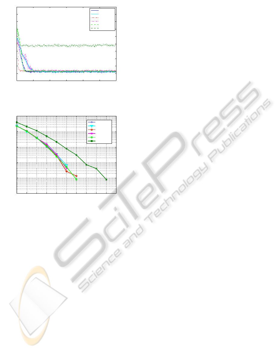
0 200 400 600 800 1000 1200
−50
−40
−30
−20
−10
0
10
20
30
40
50
samples
MSE(dB)
CG
MMax CG
RLS
MMax RLS
EDS
MMax EDS
Figure 5: Comparison of MSE of PU CG with PU RLS and
PU EDS.
5 6 7 8 9 10 11 12 13 14 15
10
−6
10
−5
10
−4
10
−3
10
−2
10
−1
SNR(dB)
SER
CG
MMax CG
RLS
MMax RLS
EDS
MMax EDS
Figure 6: Comparison of SER of PU CG with PU RLS and
PU EDS.
rithms. We use a simple short FIR channel (Sayed,
2003)
C(z) = 0.5+ 1.2z
−1
+ 1.5z
−2
− z
−3
. (46)
We assume the full length of the equalizer is 30 and
the PU length is 15. The input sequence is 4-QAM.
The results are obtained by averaging 50 independent
runs. Figure 6 illustrates the symbol-error-rate (SER)
in log-scale among CG, MMax CG, RLS, MMax
RLS, EDS, and MMax EDS algorithms. The SER
performance of these algorithms are still related to
the MSE performance shown in Figure 5. The full-
update CG, RLS, and EDS have similar SER perfor-
mance. The MMax CG and MMax RLS have simi-
lar performance, and their performance are also close
to the full-update algorithms. The MMax CG needs
2325 multiplications while the MMax RLS needs
2819 multiplications per symbol. We can see that the
MMax CG can achieve similar SER performance as
the MMax RLS, with lower computational cost. The
MMax EDS does not perform as well as the other al-
gorithms.
5 CONCLUSIONS
In this paper, different PU CG algorithms are de-
veloped. Theoretical mean and mean-square perfor-
mance are derived for white input. The performance
of different PU CG algorithms are compared by using
computer simulations. The theoretical results match
the simulated results. The performance of PU CG is
also compared with PU RLS and PU EDS. We can
conclude that the MMax CG algorithm can achieve
comparable performance as the full-update CG while
having lower computational complexity than the full-
update CG. In the future, the performance will be fur-
ther analyzed for correlated input. Other performance
such as stability and tracking performance, will also
be analyzed.
ACKNOWLEDGEMENTS
This work was supported in part by NASA grant
#NNG06GE95G, and the Institute for Critical Tech-
nology and Applied Science.
REFERENCES
Bose, T. (2004). Digital Signal and Image Processing. Wi-
ley, New York.
Chang, P. S. and Willson, A. N. (2000). Analysis of conju-
gate gradient algorithms for adaptive filtering. IEEE
Trans. Signal Processing, 48(2):409–418.
Do˘ganc¸ay, K. (2008). Partial-Update Adaptive Signal Pro-
cessing. Academic Press.
Douglas, S. C. (1995). Analysis and implementation of the
max-nlms adaptive filter. In Proc. Twenty-Ninth Asilo-
mar Conference on Signals, Systems and Computers,
pages 659–663.
Douglas, S. C. (1997). Adaptive filters employing partial
updates. IEEE Trans. Circuits and Systems II: Analog
and Digital Signal Processing, 44(3):209–216.
Godavarti, M. and Hero III, A. O. (2005). Partial up-
date lms algorithms. IEEE Trans. Signal Processing,
53(7):2382–2399.
Khong, A. W. H. and Naylor, P. A. (2007). Selective-tap
adaptive filtering with performance analysis for iden-
tification of time-varying systems. IEEE Trans. Audio,
Speech, and Language Processing, 15(5):1681–1695.
Mayyas, K. (2005). Performance analysis of the deficient
length lms adaptive algorithm. IEEE Trans. Signal
Processing, 53(8):2727–2734.
Naylor, P. A. and Khong, A. W. H. (2004). Affine projection
and recursive least squares adaptive filters employing
partial updates. In Proc. Thirty-Eighth Asilomar Con-
ference on Signal, System & Computers, pages 950–
954.
PECCS 2011 - International Conference on Pervasive and Embedded Computing and Communication Systems
322

Sayed, A. H. (2003). Fundamentals of Adaptive Filtering.
Wiley, New York.
Wu, J. and Doroslovacki, M. (2007). A mean convergence
analysis for partial update nlms algorithms. In Proc.
CISS, pages 31–34.
Xie, B. and Bose, T. (2010). Partial update EDS algorithms
for adaptive filtering. In Proc. ICASSP.
Zhang, Z. K., Bose, T., Xiao, L., and Thamvichai, R.
(2006). Performance analysis of the deficient length
EDS adaptive algorithms. In Proc. APCCAS, pages
222–226.
PARTIAL UPDATE CONJUGATE GRADIENT ALGORITHMS FOR ADAPTIVE FILTERING
323
