
METHOD OF EXTRACTING INTEREST POINTS BASED ON
MULTI-SCALE DETECTOR AND LOCAL E-HOG DESCRIPTOR
Manuel Grand-brochier, Christophe Tilmant and Michel Dhome
Laboratoire des Sciences et Matriaux pour l’Electronique, et d’Automatique (LASMEA)
UMR 6602 UBP-CNRS, 24 avenue des Landais, 63177 Beaumont, France
Keywords:
Multi-scales analysis, Local descriptor, Robustness to image transformations, Elliptical-HOG.
Abstract:
This article proposes an approach to extraction (detection and description) of interest points based Fast-Hessian
and E-HOG. SIFT and SURF are the two most used methods for this problem and their studies allow us to
understand their construction and extract the various advantages (invariances, speeds, repeatability). Our goal
is, firstly, to couple these advantages to create a new system (detector, descriptor and matching) and, secondly,
to determine the characteristic points for different applications (image transformation, 3D reconstruction...).
Our system must also be as invariant as possible for the image transformation (rotations, scales, viewpoints
for example). Finally, we have to find a compromise between a good matching rate and the number of points
matched. All the detector and descriptor parameters (orientations, thresholds, analysis shape) will be also
detailed in this article.
1 INTRODUCTION
There are a large number of applications based on im-
age analysis, especially 3D reconstruction problems,
tracking or pattern recognition for example. These ap-
plications need data usually extracted with two tools:
the detection of interest points (Li and Allison, 2008)
and the local description (Li and Allison, 2008) of
these. The detector analyses the image to extract
the characteristic points (corners, edges, blobs). The
neighborhood study allows us to create a local points
descriptor, in order to match them. For matched in-
terest points, the robustness of various transforma-
tions of the image is very important. To be robust to
scale, interest points are extracted with a global multi-
scales analysis, we considered the Harris-Laplace de-
tector (Harris and Stephens, 1988; Mikolajczyk and
Schmid, 2004b; Mikolajczyk and Schmid, 2002), the
Fast-Hessian (Bay and al., 2006) and the difference
of Gaussians (Lowe, 1999; Lowe, 2004). The de-
scription is based on a local exploration of interest
points to represent the characteristics of the neighbor-
hood. In comparative studies (Choksuriwong and al.,
2005; Mikolajczyk and Schmid, 2004a; Bauer and al.,
2007), it is shown that oriented gradients histograms
(HOG) give good results. Among the many meth-
ods using HOG, we retain SIFT (Scale Invariant Fea-
ture Transform) (Lowe, 1999; Lowe, 2004) and SURF
(Speed Up Robust Features) (Bay and al., 2006), us-
ing a rectangular neighborhood exploration (R-HOG:
Rectangular-HOG). We also mention GLOH (Gra-
dient Location and Orientation Histogram) (Mikola-
jczyk and Schmid, 2004a; Dalal and Triggs, 2005)
and Daisy (Tola et al., 2008), using circular geometry
(C-HOG: Circular-HOG). To provide the best possi-
ble list of points for different applications, we pro-
pose to create a system of detection and local de-
scription which is the most robust possible against the
various transformations that can exist between two
images (illumination, rotation, viewpoint for exam-
ple). It should also be as efficient as possible as re-
gards the matching rate. Our method relies on a Fast-
Hessian points detector, an elliptical exploration and a
local descriptor based E-HOG (Elliptical-HOG). We
propose to estimate local orientation, with the study
of the Harris matrix, in order to adjust the descrip-
tor (rotation invariance) and finally we will normalize
(brightness invariance).
Section 2 presents briefly SIFT and SURF, and
lists the advantages of each. The various tools and
their parameters (orientations, thresholds, analysis
pattern) we use are detailed in Section 3. To com-
pare our approach to SIFT and SURF, many tests have
been carried out. A synthesis of the different results
is presented in Section 4.
59
Grand-brochier M., Tilmant C. and Dhome M..
METHOD OF EXTRACTING INTEREST POINTS BASED ON MULTI-SCALE DETECTOR AND LOCAL E-HOG DESCRIPTOR.
DOI: 10.5220/0003369300590066
In Proceedings of the International Conference on Computer Vision Theory and Applications (VISAPP-2011), pages 59-66
ISBN: 978-989-8425-47-8
Copyright
c
2011 SCITEPRESS (Science and Technology Publications, Lda.)
2 RELATED WORK
In order to propose a robust method and giving many
interest points, Lowe propose a new approach, SIFT
(Lowe, 1999; Lowe, 2004), consisting of a difference
of Gaussians (DoG) and R-HOG analysis. The de-
tector is based on an approximation of the Laplacian
of Gaussian (Lindeberg, 1998) and interest points are
obtained by maximizing the DoG:
D(x, y, σ) =(G(x, y, kσ) −G(x, y, σ)) ∗I(x, y)
L(x, y, kσ) −L(x, y, σ).
(1)
The descriptor uses an orientation histogram, based
on equation 2, to determine the angle of rotation θ to
be applied to the mask analysis.
θ(x, y) = tan
−1
(
(L(x, y + 1) −L(x, y −1)
(L(x + 1, y) −L(x −1, y)
) (2)
It then uses R-HOG, formed by local gradients in the
neighborhood, previously smoothed by a Gaussian.
Finally, the descriptor is normalized to be invariant
to illumination changes.
An extension of SIFT, GLOH (Mikolajczyk and
Schmid, 2004a; Dalal and Triggs, 2005), has been
proposed to increase the robustness. It amounts to
the insertion of a grid in log polar localization. The
mask analysis of this descriptor is composed of three
rings (C-HOG), whose two largest are divided along
eight directions. More recently, the descriptor Daisy
(Tola et al., 2008) has been proposed. It is also based
on a circular neighborhood exploration and constructs
convolved orientation maps.
SIFT has not a fast computational speed. SURF
(Bay and al., 2006) proposes a new approach, whose
main objective is to accelerate the various image pro-
cessing steps. The first problem was to choose the
detector method. The various tests (Juan and Gwun,
2009; Bay and al., 2006) show that the Fast-Hessian
has the best repetability rate. It is based on the Hes-
sian matrix:
H(x, y, σ) =
L
xx
(x, y, σ) L
xy
(x, y, σ)
L
xy
(x, y, σ) L
yy
(x, y, σ)
, (3)
with L
i j
(x, y, σ) the second derivative in the directions
i and j of L. The maximization of its determinant
(Hessian) allows us to extract the coordinates of in-
terest points in a given scale. The second step, the
local description, is based on Haar wavelets. These
estimate the local orientation of the gradient, allow-
ing the construction of the descriptor. Finally, SURF
studied the sign of the wavelet transform to increase
the quality of results.
The presented methods use similar tools: multi-
scale analysis (Fast-Hessian or DoG), local descrip-
tion based HOG, local smoothing and descriptor nor-
malization. For matching they use a minimization
of either the Euclidean distance between descrip-
tors (SURF) or the angle between vectors descriptors
(SIFT). Many tests (Mikolajczyk and Schmid, 2004a;
Juan and Gwun, 2009; ?) can establish a list of dif-
ferent qualities of each. It follows that SURF, with
its detector, has the best repeatability for viewpoint
changes, scale, noise and lighting. It is also faster
than SIFT, however it has a higher precision rate for
rotations and scale changes. It has also a higher num-
ber of detected points for all transformations. It might
be interesting to combine these two methods.
3 METHOD
The method we propose is divided into three parts: a
Fast-Hessian multi-scale detector, a local E-HOG de-
scriptor and an optimized matching. This section de-
scribes the different steps of our method and param-
eters used. The detector Fast-Hessian provides a list
of interest points, characterized by their coordinates
and local scale. Our descriptor is based on the Harris
matrix interpretation, and the construction of E-HOG.
Matching is based on an approximation of the nearest
neighbors and removing duplicates. These issues will
be detailed below.
3.1 Detection
The Fast-Hessian is an approximated method of Hes-
sian matrix (equation 3), to reduce the computing
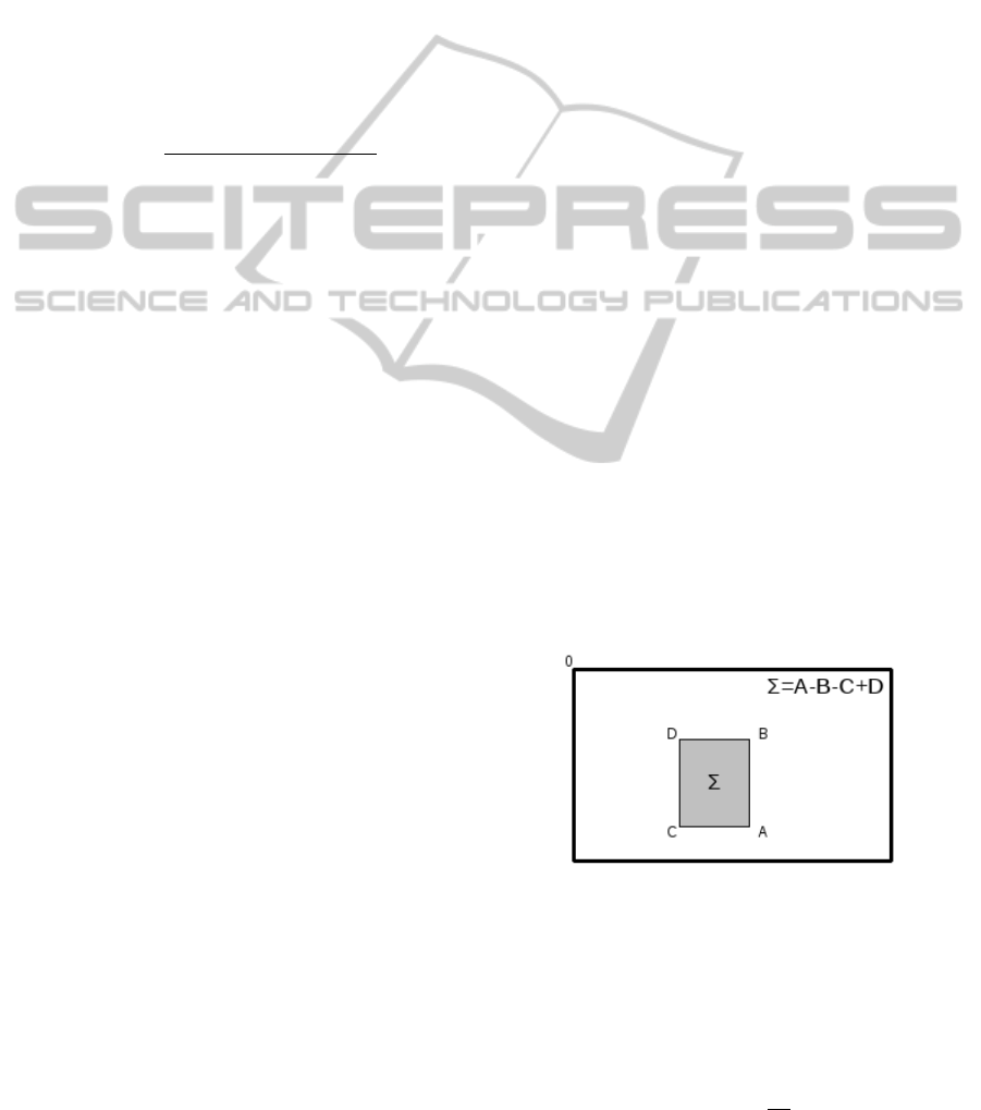
time. This detector uses integral images (Figure 1),
therefore it takes only three additions and four mem-
ory accesses to calculate the sum of intensities inside
a rectangular region of any size. The Fast-Hessian
Figure 1: Determination of integral image.
relies on the exploitation of the Hessian matrix (equa-
tion 3), whose determinant is calculated as follows:
det(H(x, y, σ)) =
σ
2
(L
xx
(x, y, σ)L
yy
(x, y, σ) −L
2
xy
(x, y, σ)),
(4)
where L
xx
(x, y, σ) is the convolution of the Gaus-
sian second order derivative
∂
2
∂x
2
g(σ) with the im-
VISAPP 2011 - International Conference on Computer Vision Theory and Applications
60
age I in point (x, y), and similarly for L
xy
(x, y, σ) and
L
yy
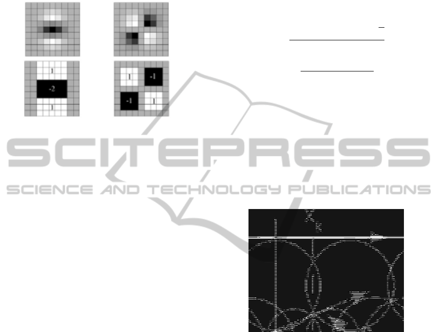
(x, y, σ). Gaussians are optimal for scale-space
analysis and the Fast-Hessian provides an approxima-
tion of these second order derivative (Figure 2).
Figure 2: Top row: Gaussian second order partial deriva-
tives, bottom row: approximation for the second order
Gaussian partial derivatives.
By looking for local maxima of the determinant,
we establish a list of K points associated with a scale,
denoted {(x
k
, y
k
, σ
k
); k ∈[[0;K −1]]}, where:
(x
k
, y
k
, σ
k
) = argmax
{x,y,σ}
(det(H(x, y, σ))). (5)
The number of interest points obtained depends on the
space scale explored and thresholding of local max-
ima. We have to find a compromise between scale
space exploration and relevance of extracted points.
The influence of this one will be detailed in Section 4.
3.2 Description
As with SIFT and SURF, our method is based on
HOG, yet our analysis window will consist of ellipses
(E-HOG). Different tools will also be necessary to ad-
just and normalize our descriptor.
3.2.1 Determining the Local Orientation
Gradient
To be as invariant as possible for rotations, estimat-
ing the local orientation gradient of the interest point
is necessary. This parameter allows us to adjust the
E-HOG, giving an identical orientation for two corre-
sponding points. For this, we use the Harris matrix,
calculated for each point (x
k
, y
k
) and defined by:
M
H
(x
k
, y
k
) =
"
∑
V (x
k
,y
k
)
[I
x
(x
k
, y
k
)]
2
∑
V (x
k
,y
k
)
I
x
(x
k
, y
k
)I
y
(x
k
, y
k
)
∑
V (x
k
,y
k
)
I
x
(x
k
, y
k
)I
y
(x
k
, y
k
)
∑
V (x
k
,y
k
)
[I
y
(x
k
, y
k
)]
2
#
(6)
where V (x
k
, y
k
) represents the neighborhood of the in-
terest point, I
x
and I
y
are the first derivatives in x and
y of image, calculated using the Canny-Deriche oper-
ator. The properties of this matrix can study the infor-
mation dispersion. The local analysis of its eigenvec-
tors (
−→
v
1
and
−→
v
2
) associated with corresponding eigen-
values can extract an orientation estimate:
∆ = Trace(M
H
(x
k
, y
k
))
2
−4Det(M
H
(x
k
, y
k
))
λ
1
=
Trace(M
H
(x
k
, y
k
)) +
√
∆
2
−→
v
1
=
(
∑
V (x
k
,y
k
)
[I
y
(x
k
,y
k
)]
2
)−λ
1
∑
V (x
k
,y
k
)
I
x
(x
k
,y
k
)I
y
(x
k
,y
k
)
1
θ
k
= arctan(
−→
v
1
). (7)
3.2.2 Descriptor Construction
The initial shape of our descriptor relies on a circular
neighborhood exploration of the interest point. The
seventeen circles used, are divided into three scales
(Figure 3) and are adjusted by θ
k
(equation 7).
Figure 3: Initial mask analysis of our descriptor, centered at
(x
k
, y
k
) and oriented by an angle θ
k
.
This angle allows us to be robust to image rotation.
The circle diameter is proportional to σ
k
, thus accen-
tuating the scale invariance. To manage the prob-
lem of viewpoint changes and anisotropic transforma-
tions, we propose to modify the shape of our descrip-
tor. The goal is to get local information more consis-
tently. We propose to use an elliptical exploration to
describe the neighbor of interest points (Figure 4).
An analysis of the properties of affine detectors
(Mikolajczyk and Schmid, 2004b; Mikolajczyk and
al., 2005) allows us to determine the ratio r
k
between
the axes of ellipses. For example for the Harris affine
detector, two scales are used and are bound by the
following equation: σ
k
D
= sσ
k
I
where σ
D
is the differ-
entiation scale, σ
I
is the integration scale and s is the
ratio. It is noted that s is generally between 0.5 and
METHOD OF EXTRACTING INTEREST POINTS BASED ON MULTI-SCALE DETECTOR AND LOCAL E-HOG
DESCRIPTOR
61
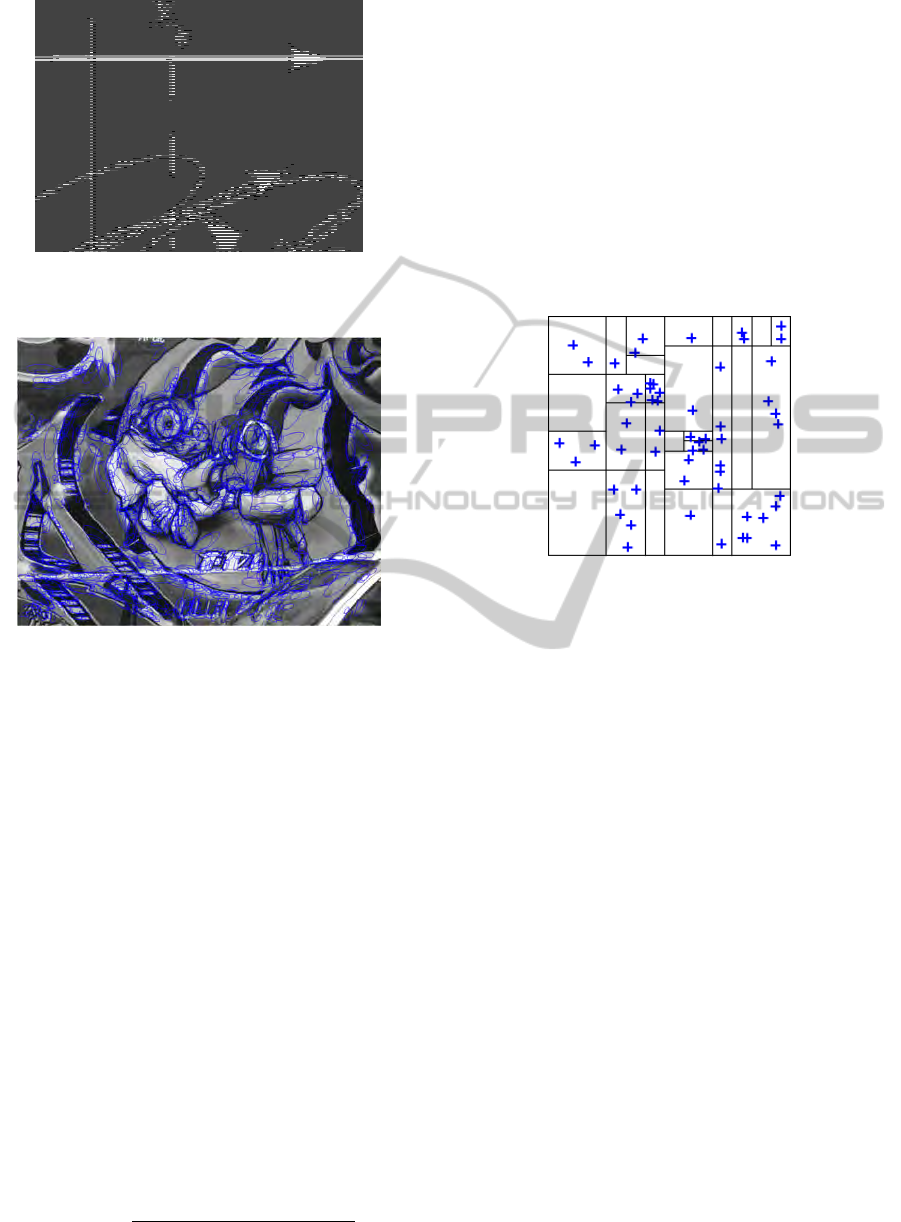
Figure 4: Final mask analysis of our descriptor, centered at
(x
k
, y
k
) and oriented by an angle θ
k
.
Figure 5: Example of local description of interest points.
0.75. By the parallelism between these two scales and
our ellipses, it is possible to determine the best ratio
r
k
. Based on many tests, the ratio giving the best re-
sult is equal to 0.5. Figure 5 illustrates the construc-
tion of our ellipses (for better visualization, we only
show the central ellipse of each descriptor).
We construct a HOG eight classes (in steps of 45)
for each ellipse. Our descriptor, we note des
I
(x
k
, y
k
),
belongs to R
136
(17 ellipses × 8 directions). To be
invariant for brightness changes, histogram is normal-
ized and we use also a threshold for E-HOG to remove
the high values of gradient.
3.3 Matching
The objective is to find the best similarity (corre-
sponding to the minimum distance) between descrip-
tors of two images. Euclidean distance, denoted d
e
,
between two descriptors is defined by:
d
e
(des
I
1
(x
k
,y
k
), des
I
2
(x
l
, y
l
)) =
q
[des
I
1
(x
k
, y
k
)]
T
·des
I
2
(x
l
, y
l
).
(8)
The minimization of d
e
, denoted d
min
, provides a pair
of points {(x
k
, y
k
);(x
˜
l
, y
˜
l
)}:
˜
l = argmin
l∈[[0;L−1]]
(d
e
(des
I
1
(x
k
, y
k
), des
I
2
(x
l
, y
l
))), (9)
d
min
= d
e
(des
I
1
(x
k
, y
k
), des
I
2
(x
˜
l
, y
˜
l
)). (10)
To simplify the search for this minimum distance,
we propose to use an approximative nearest neigh-
bor search method (a variant of k-d tree) (Arya and
al., 1998). The principle is to create a decision tree
based on descriptors components of the second image
(Figure 6). So, for each new descriptor of the first im-
Figure 6: Example of decision tree to extract the nearest
neighbors.
age, all components are tested and the nearest neigh-
bor is defined. Research is therefore faster, without
sacrificing precision. To have a more robust match-
ing, thresholding is applied to this distance, to find a
``high´´minimum. The pair of points is valid if:
d
min
≤ α ×min(d
e
(des
1
(x
k
, y
k
), des
2
(x
l
, y
l
))), (11)
for l ∈[[0; N −1]]\
˜
l and with α the threshold selection
(detailed in Section 4). We do not allow a point to
match with several other points, and a final step is to
remove duplicates.
4 RESULTS
We are going to compare our method with SIFT and
SURF. These two methods are the most used and give
the best results. We propose to study the matching
rate and the precision of each of them. We will also
study the recall = f (1 −precision) curves and the es-
timation error of the transformed image.
4.1 Databases
To validate our method, we chose two databases:
VISAPP 2011 - International Conference on Computer Vision Theory and Applications
62
• The first one, noted ODB and extracted from the
Oxford
1
database, proposes scene transforma-
tions with an access to the matrix of homography.
Transformations studied are brightness changes
(ODB
b
), modified jpeg compressions (ODB
c
),
blur (ODB
n
), rotations and scales (ODB
rs
), and
small and large angle viewpoint changes (respec-
tively ODB
vs
and ODB
vl
). Figure 7 illustrates this
database.
ODB
b
ODB
c
ODB
n
ODB
rs
ODB
vs
ODB
vl
Figure 7: Examples of images used for transformations:
(top: left to right) brightness changes, modified jpeg com-
pressions, blur, (bottom: left to right) rotations + scales,
viewpoint changes (small angle), and viewpoint changes
(large angle).
• A second database, noted SDB, composed of a
set of synthetic image transformations (Figure 8
and Figure 9). These transformations are rota-
tions 45 (SDB
r
), scales (SDB
s
), anisotropic scales
(SDB
as
), rotations 45 + scales (BS
rs
) and rotations
45 + anisotropic scales (BS
ras
).
SDB
r
SDB
r
SDB
s
Figure 8: Examples of laboratory images (board cameras)
used for synthetic transformations.
1
http://www.robots.ox.ac.uk/∼vgg/data/data-aff.html
SDB
as
SDB
ras
SDB
rs
Figure 9: Examples of internet images (Pig, Lena, Beatles)
used for synthetic transformations.
4.2 The Parameters of our Method
4.2.1 Influence of the Number of Octave
(Detection Parameter)
To get the best compromise between relevance and
number of extracted points, we use the following
curves:
Figure 10: These graphs represent, for ODB
vl
images: (top)
the correct matching rate according to the number of octave
and (bottom) the number of points that can be matched.
It represents, on one hand the matching precision
for ODB
vl
images, on the other hand the number of
points that can be matched. The best compromise is
two octaves, it has better precision than three or four
octaves while keeping an almost identical number of
points. One octave has a better precision than two
octaves, but loses a lot of points. Therefore we choose
two octaves instead of four used by SURF.
4.2.2 Threshold Selection
The threshold selection α used in the equation 11 is
determinated by analysing the curves of Figure 11.
This threshold allows us to increase the selectivity,
METHOD OF EXTRACTING INTEREST POINTS BASED ON MULTI-SCALE DETECTOR AND LOCAL E-HOG
DESCRIPTOR
63
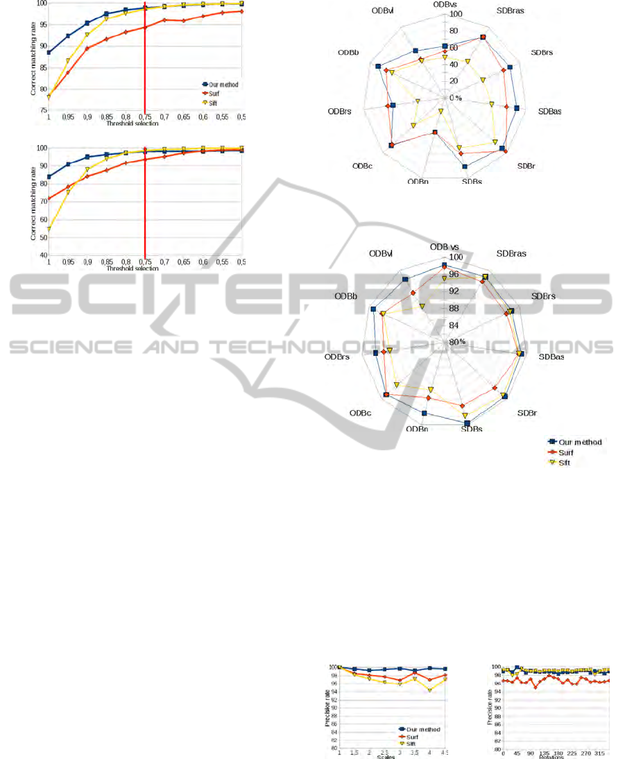
Figure 11: These graphs represent the correct matching rate
according to the threshold selection. Top is for viewpoint
changes (grafiti 1 → 2) and bottom is for rotation + scale
(boat 1 → 3).
but the consequence is a reduction in the number of
matched points.
If the threshold goes away from 1, the matching
becomes more selective and therefore fewer points are
used. The problem is to find the best compromise be-
tween the correct matching rate and the number of
matched points. SIFT recommands a threshold of 0.8
and SURF a threshold of 0.7. By analysing curves of
Figure 11, we choose a threshold α = 0.75.
4.3 Evaluation Tests and Results
4.3.1 Matching Rate and Precision
We propose to compare the matching rate T
a
, as well
as the precision P of every method. T
a
is defined by
the number of correct matches divided by the num-
ber of possible matches. P is defined by the number
of correct matches divided by the number of matches
performed. A synthesis of the results obtained is pro-
posed in Figure 12.
Our method presents results better or as good as
SIFT and SURF. Our matching rate remains better
than the two other methods with the exception of the
databases ODB
rs
and SDB
r
transformations. Never-
theless the difference between SURF and our method
for this type of transformation is lower than 4%. For
other type of transformation, the biggest differences
are observed for rotation 45 + scale (≈ 10% between
our method and SURF and 37% with SIFT) and for
large angle viewpoint changes (≈ 18% with SURF
and SIFT). Our matching precision is also better and
T
a
P
Figure 12: These graphs represent at top: a matching rate
and at bottom: a matching precision. Matching rate is the
ability to match points and matching precision is the match
quality. The goal is to have the highest rate of correctly
matched points (with better precision).
remains constantly above 95%. The biggest differ-
ence is obtained for large angle viewpoint changes
(4% for SURF and 8% for SIFT). To detail the preci-
sion curves of different methods, we propose graphs
in Figures 13 to 16.
(a) (b)
Figure 13: (a) precision rate for scales changes (SDB
s
) and
(b) precision rate for rotations (SDB
r
).
These curve show a better precision rate for our
method, or similar for rotation transformations (figure
VISAPP 2011 - International Conference on Computer Vision Theory and Applications
64
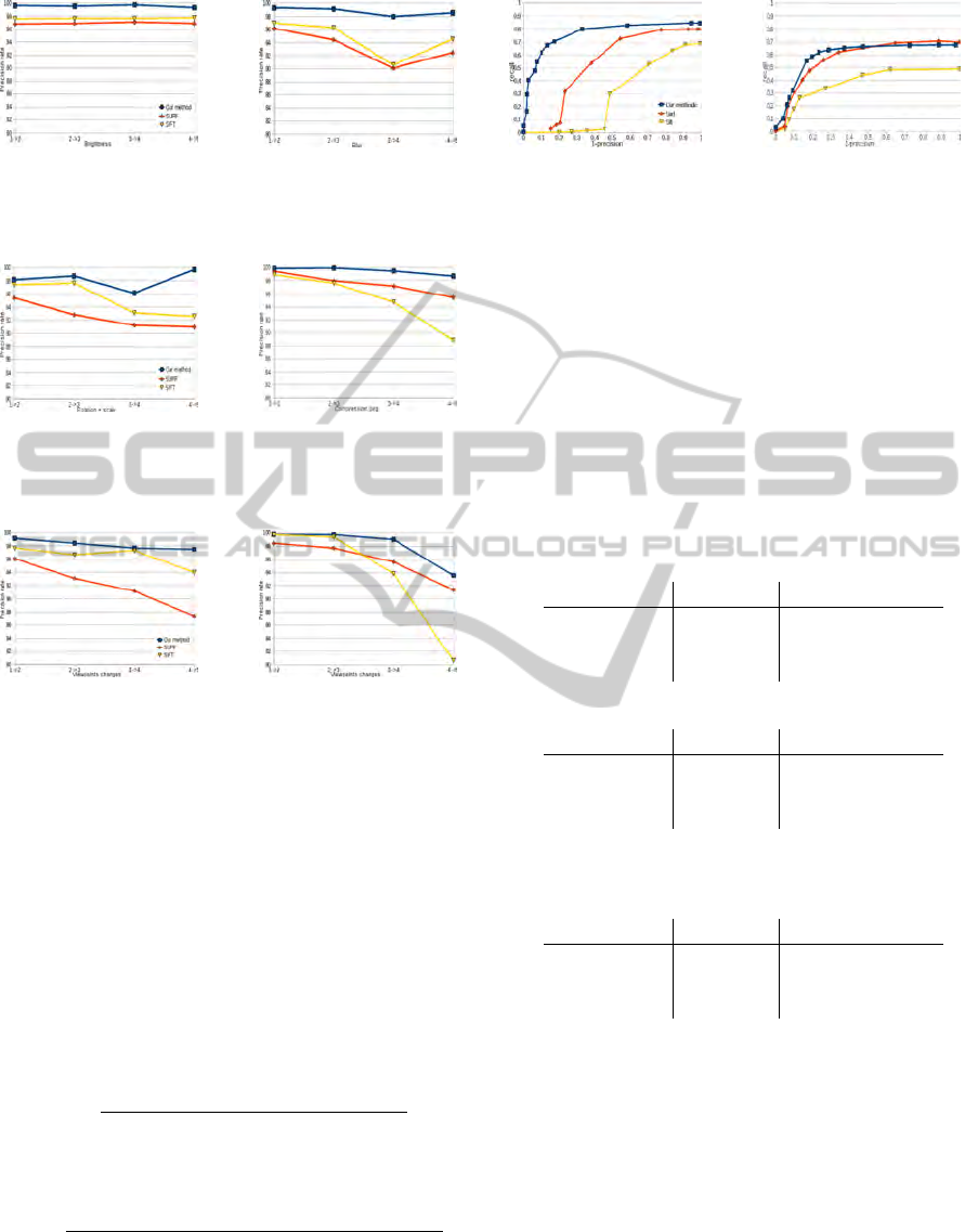
(a) (b)
Figure 14: (a) precision rate for brightness (ODB
b
) and (b)
precision rate for blur (ODB
n
).
(a) (b)
Figure 15: (a) precision rate for rotation and scale (ODB
rs
)
and (b) precision rate for compression jpeg (ODB
c
).
(a) (b)
Figure 16: (a) and (b) precision rate for viewpoints changes
respectively (ODB
vl
) and (ODB
vs
).
13.b). Another observation can be made through the
transformations studied, concerning the stability of
our method. Indeed, our curves decrease more slowly
than SIFT and SURF, implying a precision rates more
constant.
4.3.2 Influence of Data
To observe the influence of data on different methods,
we use the recall = f (1 −precision) curves (Mikola-
jczyk and Schmid, 2004a) with two components come
from:
recall =
number of correct matches
number of possible correct matches
,
and
1 −precision =
number of false matches
number of (correct matches + false matches
.
We propose to analyse two curves (Figure 17) and we
can observe that our method is more stable than SIFT
and SURF. Therefore, our method is more robust to
the deterioration of data for these transformations.
(a) (b)
Figure 17: (a) a recall versus 1-precision for brightness
(ODB
b
: 1→ 4) and (b) a recall versus 1-precision for ro-
tation + scale (ODB
rs
: 2→ 4).
4.3.3 Estimation of the Image Transformation
We propose a final study on the estimation of the ho-
mography matrix. For 3D reconstruction, for exam-
ple, the estimate of this matrix is very important, and
the goal is to have the best estimation (the error as low
as possible) with maximum points validating this ma-
trix. The estimation is based on the matches and the
Ransac algorithm. We studied three transformations
and the results are:
• viewpoints changes (ODB
vl
):
error (%) valid points (%)
Our method 0.06 96.72
SURF 3.46 96.34
SIFT 2.98 92.35
• rotation and scale (ODB
rs
):
error (%) valid points (%)
Our method 0.54 93.23
SURF 1.69 86.03
SIFT 2.06 88.24
• blur (ODB
n
):
error (%) valid points (%)
Our method 0.61 97.13
SURF 0.66 92.1
SIFT 0.58 96.56
Our method obtains, for the first two transformations,
an error rate below SIFT and SURF and a higher rate
of valid points. For the last transformation, the results
are similar for all three methods.
5 CONCLUSIONS
In this article we presented a method based on, on the
one hand the avantages of SIFT and SURF (repetabil-
ity, invariances) and on the other hand the use of tools
such as the Harris matrix, the HOG or the decision
tree. Detection relies on Fast-hessian detector that we
METHOD OF EXTRACTING INTEREST POINTS BASED ON MULTI-SCALE DETECTOR AND LOCAL E-HOG
DESCRIPTOR
65

thresholded. Description interprets the Harris matrix
and uses an elliptical shape to adapt the descriptor
to the image transformation. Finally, matching cre-
ates decision tree and removes duplicates. To vali-
date our method, we compared it to SIFT and SURF.
Our method has better matching rate and better preci-
sion for most transformations. It is also robust to data
degradation problems and provides an estimation of
homography matrix more reliable, keeping good rate
of valid points. Therefore data extracted from im-
ages are better and will result in an improvement of
the applications referred (3D reconstruction or pattern
recognition for example).
Our prospects are a generalization of our method,
with application to a spatio-temporal analysis. We
will add a temporal variable to the Hessian matrix
(equation 3). We also transform our descriptor shape
to obtain an neighborhood exploration ellipsoidal (for
tracking for example). An other prospect is to inte-
grate a third dimension to use it in medical imaging.
REFERENCES
Arya, S., Mount, D., Netanyahu, N., Silverman, R., and
Wu, A. (1998). An optimal algorithm for approxi-
mate nearest neighbor searching in fixed dimensions.
J.ACM, 45:891–923.
Bauer, J., Snderhauf, N., and Protzel, P. (2007). Compar-
ing several implementations of two recently published
feature detectors. Intelligent Autonomous Vehicles.
Bay, H., Tuylelaars, T., and Gool, L. V. (2006). Surf :
Speeded up robust features. European Conference on
Computer Vision.
Choksuriwong, A., Laurent, H., and Emile, B. (2005).
Etude comparative de descripteur invariants d’objets.
ORASIS.
Dalal, N. and Triggs, B. (2005). Histograms of oriented
gradients for human detection. IEEE Conference on
Computer Vision and Pattern Recognition.
Harris, C. and Stephens, M. (1988). A combined corner and
edge detector. Alvey Vision Conference, pages 147–
151.
Juan and Gwun (2009). A comparison of sift, pca-sift
and surf. International Journal of Image Processing,
3(4):143–152.
Li, J. and Allison, N.M. (2008). A Comprehensive Review
of Current Local Features for Computer Vision. Neu-
rocomputing, 71(10-12):1771–1787.
Lindeberg, T. (1998). Feature detection with automatic
scale selection. International Journal of Computer Vi-
sion, 30(2):79–116.
Lowe, D. (1999). Object recognition from local scale-
invariant features. IEEE International Conference on
Computer Vision, pages 1150–1157.
Lowe, D. (2004). Distinctive image features from scale-
invariant keypoints. International Journal of Com-
puter Vision, 60(2):91–110.
Mikolajczyk, K., and Schmid, C. (2002). An affine invari-
ant interest point detector. European Conference on
Computer Vision, 1:128–142.
Mikolajczyk, K. and Schmid, C. (2004a). A performance
evaluation of local descriptors. IEEE Pattern Analysis
and Machine Intelligence, 27(10):1615–1630.
Mikolajczyk, K., Tuytelaars, T., Schmid, C., Zisserman, A.,
Matas, J., Schaffalitzky, F., Kadir, T., and Van Gool, L.
(2005). A comparaison of affine region detectors. In-
ternational Journal of Computer Vision, 65(1/2):43–
72.
Mikolajczyk, K. and Schmid, C. (2004b). Scale & affine in-
variant interest point detectors. International Journal
of Computer Vision, 1(60):63–86.
Tola, E., Lepetit, V., and Fua, P. (2008). A fast local descrip-
tor for dense matching. IEEE Conference on Com-
puter Vision and Pattern Recognition.
VISAPP 2011 - International Conference on Computer Vision Theory and Applications
66
