
FAST LEARNABLE OBJECT TRACKING AND DETECTION IN
HI
GH-RESOLUTION OMNIDIRECTIONAL IMAGES
David Hurych, Karel Zimmermann and Tom´aˇs Svoboda
Center for Machine Perception, Department of Cybernetics
Faculty of Electrical Engineering, Czech Technical University in Prague, Prague, Czech Republic
Keywords:
Detection, Tracking, Incremental, Learning, Predictors, Fern, Omnidirectional, High-resolution.
Abstract:
This paper addresses object detection and tracking in high-resolution omnidirectional images. The foreseen
application is a visual subsystem of a rescue robot equipped with an omnidirectional camera, which demands
real time efficiency and robustness against changing viewpoint. Object detectors typically do not guarantee
specific frame rate. The detection time may vastly depend on a scene complexity and image resolution. The
adapted tracker can often help to overcome the situation, where the appearance of the object is far from the
training set. On the other hand, once a tracker is lost, it almost never finds the object again. We propose a
combined solution where a very efficient tracker (based on sequential linear predictors) incrementally accom-
modates varying appearance and speeds up the whole process. We experimentally show that the performance
of the combined algorithm, measured by a ratio between false positives and false negatives, outperforms both
individual algorithms. The tracker allows to run the expensive detector only sparsely enabling the combined
solution to run in real-time on 12 MPx images from a high resolution omnidirectional camera (Ladybug3).
1 INTRODUCTION
This paper focuses on the problem of real-time ob-
ject detection and tracking in a sequence of high-
resolution omnidirectional images. The idea of com-
bining a detector and fast alignment by a tracker has
already been used in several approaches (Li et al.,
2010; Hinterstoisser et al., 2008). The frame rate
of commonly used detectors naturally depends on
both the scene complexity and image resolution. For
example, the speed of ferns (
¨
Ozuysal et al., 2010),
SURF (Bay et al., 2006) and SIFT (Lowe, 2004) de-
tectors depends on the number of evaluated features,
which is generally proportional to the scene complex-
ity (e.g. number of Harris corners) and image resolu-
tion. The speed of Waldboost (
ˇ
Sochman and Matas,
2005) (or any cascade detector) depends on the num-
ber of computations performed in each evaluated sub-
window. In contrast, most of the trackers are inde-
pendent of both the scene complexity and image res-
olution. This guarantees stable frame rate however,
once the tracker is lost it may never recover the ob-
ject position again. Adaptive trackers can follow an
object which is far from the training set and cannot be
detected by the detector. We propose to combine a de-
tector and a tracker to benefit from robustness (ability
to find an object) of detectors and locality (efficiency)
Figure 1: Omnidirectional high resolution image (12 Mpx)
c
aptured by Ladybug 3 camera. Three objects are marked.
of trackers.
Ferns-based detector (also used by (Hinterstoisser
et al., 2008) for 10 fps tracking-by-detection)is one of
the fastest object detectors because of the low number
of evaluated binary features on detected Harris cor-
ners. The speed makes the ferns detector ideal for the
purpose of object detection in large images.
One of the most popular template trackers is the
KLT tracker (Shi and Tomasi, 1994), which uses the
Lucas-Kanade gradient descent algorithm (Lucas and
Kanade, 1981). The algorithm has become very pop-
ular and has many derivations (Baker and Matthews,
2004). The gradient descent is a fast algorithm yet,
it has to compute the image gradient, the Jacobian
and inverse Hessian of the modeled warp in every
frame. For some simple warps, the Jacobian may
521
Hurych D., Zimmermann K. and Svoboda T..
FAST LEARNABLE OBJECT TRACKING AND DETECTION IN HIGH-RESOLUTION OMNIDIRECTIONAL IMAGES.
DOI: 10.5220/0003369705210530
In Proceedings of the International Conference on Computer Vision Theory and Applications (VISAPP-2011), pages 521-530
ISBN: 978-989-8425-47-8
Copyright
c
2011 SCITEPRESS (Science and Technology Publications, Lda.)

be precomputed (Hager and Belhumeur, 1998), (Del-
laert and Collins, 1999). One may also get a rid
of the inverse Hessian computation by switching the
roles of the template and image (Baker and Matthews,
2004). Nevertheless we always need to compute the
image gradients and in general case also the Jacobian
and inverse Hessian of the warp. An alternative for
template tracking are regression-based methods (Ju-
rie and Dhome, 2002), (Zimmermann et al., 2009a).
They avoid the computation of image gradient, Ja-
cobian and inverse Hessian by learning a regression
matrix from training examples. Once learned they es-
timate the tracking parameters directly from the im-
age intensities. If the regression function is linear, it
is called linear predictor. The training phase is the
biggest disadvantage of linear predictors, because the
tracking cannot start immediately. Nevertheless, the
regression matrix (function) may be estimated only
from one image in a short time (few seconds). The
training examples are generated by random warpings
of the object template and collecting image intensi-
ties. This regression matrix may be updated by ad-
ditional training examples during tracking (Hinter-
stoisser et al., 2008).
Recently, it has been shown (
¨
Ozuysal et al.,
2010), (Hinterstoisser et al., 2008), that taking advan-
tage of the learning phase, greatly improves the track-
ing speed and makes the tracker more robust with re-
spect to large perspective deformations. A learned
tracker is able to run with fragment of processing
power and estimates object position in complicated
or not yet seen poses. However, once the tracker gets
lost it may not recover the object position.
To fulfill the real-time requirements, we propose a
combination of a robust detector and a very efficient
tracker. Both, the detector and the tracker, are trained
from image data. The tracker gets updated during the
tracking. The tracker performance is extremely fast
and as a result of that, faster than real-time tracking
allows for multiple object tracking.
1.1 Related Work
We use a similar approach to (Hinterstoisser et al.,
2008), who also use a fern object detector and a linear
predictor with incremental learning for homography
estimation. The detector is used for object localiza-
tion and also for a rough estimation of patch transfor-
mation. The initial transformation is further refined
by the linear predictor, which predicts full 2D homog-
raphy. The precision of the method is validated by
inverse warping of the object patch and correlation-
based verification with the initial patch. The detec-
tor is run in every frame of the sequence of 0.3 Mpx
images processing 10 frames per second (fps). This
approach however, would not be able to perform in
real-time on 12 Mpx images. We use the fern de-
tector to determine tentative correspondences and we
run RANSAC on detected points to estimate the affine
transformation. After a positive detection we apply
the learned predictor in order to track the object for as
many frames as possible. (Hinterstoisser et al., 2008)
use an iterative version of linear predictor similar to
the one proposed by (Jurie and Dhome, 2002), while
we use SLLiP version. The SLLiP proved (Zimmer-
mann et al., 2009a) to be faster than the iterative ver-
sion, while keeping the high precision of the esti-
mation. Our tracker is incrementally updated during
tracking (Hinterstoisser et al., 2008; Li et al., 2010).
We validate the tracking by the updated tracker it-
self (see Section 2.2), which is more precise, than
correlation-based verification by a single template in
case of varying object appearance.
Recently (Holzer et al., 2010) used adaptive linear
predictors for real-time tracking. Adaptation is done
by growth or reduction of the tracked patch during
tracking and update of the regression matrices. How-
ever, this approach is not suitable for our task, because
of the need to keep in memory the large matrix with
training examples, which is needed for computation
of the template reduction and growth. This training
matrix grows with additional training examples col-
lected for on-line learning, which is undesirable for
long-term tracking.
(Li et al., 2010) use linear predictors in the form
of locally weighted projection regressors (LWPR) as
a part of self-tuning particle filtering (ISPF) frame-
work. They approximate a non-linear regression by a
piece-wise linear models. In comparison we use a se-
quence of learnable linear predictors (SLLiP) similar
to (Zimmermann et al., 2009b), which uses the result
of previous predictors in sequence as the starting point
for another predictor in a row. In (Li et al., 2010) the
partial least-squares is used for data dimension reduc-
tion. We use a subset of template pixels spread over
the object in regular grid, which proved to be suffi-
cient for dimensionality reduction, while keeping the
high precision and robustness of tracking.
The rest of this paper is organized as follows. In
Section 2 you find the formal descriptions of used
ferns detector and sequential predictor tracker and in
Section 2.3 the outline of our algorithm. In Section 3
we present the general evaluation of our algorithm.
A detailed evaluation of the detector and tracker are
given in Sections 3.1 and 3.2. In the last two sections
we discuss the computational times of the algorithm
and conclude the paper.
VISAPP 2011 - International Conference on Computer Vision Theory and Applications
522

2 THEORY
The method combines a fern-based detector and a
tracker based on sequential linear predictors. Both
the detector and the tracker are trained from the image
data. The tracker has its own validation and is incre-
mentally re-learned as the tracking goes. The detector
locates the object in case the tracker gets lost.
2.1 Ferns-based Detector
Object is modeled as a spatial constellation of de-
tected harris corners on one representativeimage. In a
nutshell: the fern detector first estimates similarity be-
tween harris corners detected in the current frame and
harris corners on the model. The thresholded similar-
ity determines tentative correspondences, which are
further refined by RANSAC selecting the largest ge-
ometrically consistent subset (i.e. set of inliers). In
our approach object was modeled as a plane. Since
we observed that the estimation of full homography
transformation was often ill-conditioned, because of
both insufficient number of detected corners and non-
planarity of the object, the RANSAC searches for the
affine transformation, which showed to be more ro-
bust.
Detailed description of the similarity measure is
in (
¨
Ozuysal et al., 2010). In the following, we pro-
vide just short description for the sake of complete-
ness. The similarity measures probability p(V(v),w)
that the observed appearance of the neighbourhood
V(v) of the detected corner v corresponds to the
model corner w. The appearance is represented as
a sequence of randomly selected binary tests, i.e.
given the corner v and sequence of n point pairs
{(x
1
,y
1
),(x
2
,y
2
),...(x
n
,y
n
)}, the appearance of the
v is encoded as binary code V
k
(v) = I(v + x
k
) >
I(v+ y
k
), where I(v+ x
k
) is the image intensity.
On one hand, it is insuficient to model probabili-
ties of binary tests independently, i.e. assuming that
p(V(v),w) =
∏
n
k=1
p
k
(V
k
(v),w). On the other hand,
modeling p(V(v),w) = p(V
1
(v),... ,V
n
(v),w) is ill-
conditioned, since we would have to estimate proba-
bility in 2
n
bins, where n is usually equal to several
hundreds. Therefore, we divide the sequence of n
binary tests into N = n/m subsequences with length
m ≈ 8 − 11. Subsequences are selected by N mem-
bership functions I(1). . . I(N) and we denote h
k
=
card(I
k
), k = 1...N. Finally, we consider these sub-
sequences to be statistically independent and model
the probability as:
p(V(v),w) =
N
∏
k=1
p
k
(V
I
k
(1)
(v),
...,V
I
k
(h
k
)
(v),w) (1)
The proposed detector requires an off-line training
phase, within which the subsequent probabilities are
estimated. Once the probabilities are pre-computed,
we use them on-line to determine the tentative corre-
spondences. In the following both phases are detailed.
Offline Training Phase. First n binary tests are ran-
domly selected and divided into N subsequences. The
model is estimated from one sample image, where
Harris corners are detected within delineated ob-
ject border. Appearance of each corner’s neighbour-
hood is modeled by N h
k
-dimensional binary hyper-
cubes, with 2
h
k
bins, representing joint probability
p
k
(V
I
k
(1)
(v),... ,V
I
k
(h
k
)
(v),w). To estimate values of
the probability, each corners neighbourhood is L-
times perturbated within the range of local deforma-
tions we want to cope with. For each perturbed train-
ing sample and each subsequence, binary tests are
evaluated and correspoding bin is increased by 1/L.
Note that different Harris corners are modeled via dif-
ferent probabilities but the same binary tests, which
allows significant improvement in the online running
phase, since the computational complexity of the sim-
ilarity computation is almost independent of the num-
ber of Harris corners on the model.
Online Running Phase. Given an input image, Harris
corners are detected. For each corner v, binary tests
are evaluated and similarity to each model corner is
computed via Equation 1. Similarities higher than a
chosen threshold determine tentative correspondeces.
Eventually, RANSAC estimates affine transformation
between model and the given image. Confidence of
the detection is equal to the number of inliers.
2.2 Sequential Linear Predictors
We extend the anytime learning of the Sequential
Learnable Linear Predictors (SLLiP) by (Zimmer-
mann et al., 2009b) in order to predict not only trans-
lation but also the full homography transformation.
Next extension is the incremental learning of new ob-
ject appearances also used by (Hinterstoisser et al.,
2008). The predictor essentially estimates deforma-
tion parameters directly from image intensities. It re-
quires a short offline learning stage before the track-
ing starts. The learning stage consists of generating
exemplars and estimation of regression functions. We
use a simple cascade of 2 SLLiPs - first for 2D motion
estimation (2 parameters) and second for homography
estimation (8 parameters). The homography is pa-
rameterized by position of 4 patch corners. Knowing
the corners position and having the reference coor-
dinates, we compute the homography transformation
for the whole patch. We have experimentally verified,
FAST LEARNABLE OBJECT TRACKING AND DETECTION IN HIGH-RESOLUTION OMNIDIRECTIONAL
IMAGES
523

that this 2-SLLiP configuration is more stable than us-
ing just one SLLiP to predict homography. First the
translation is roughly estimated by first SLLiP and
than a precise homography refinement is done. Be-
cause of speed, we opted for least squares learning
of SLLiPs similarly, as suggested by (Zimmermann
et al., 2009b).
Lets denote the translation parameters
vector t
t
= [∆x,∆y]
T
, estimated by the first
SLLiP, and the homography parameters vector
t
a
= [∆x
1
,∆y
1
,... , ∆x
4
,∆y
4
]
T
, estimated by the sec-
ond SLLiP which represents the motion of 4 object
corners c
i
= [x
i
,y
i
]
T
,i = 1,...,4. The object point
x = [x,y]
T
from previous image is transformed to
corresponding point x
′
in current image accordingly
p = A
x
1
+
t
t
0
(2)
x
′
= [p
x
/p
z
, p
y
/p
z
]
T
, (3)
where p are homogeneous coordinates. The ho-
mography matrix A is computed from 4-point cor-
respondences, between shifted object corners c
i
+ t
t
from previous image and current corners positions
c
i
+ t
t
+
t
a
2i−1
,t
a
2i
T
,i = 1,. . . ,4 estimated by the 2-
SLLiP tracker.
Estimation of parameters vectors t
t
and t
a
, learn-
ing and incremental learning will be explained for a
single SLLiP with general parameters vector t. Equa-
tions are valid for both SLLiPs, which we use. SLLiP
is simply a sequence of linear predictors. Predic-
tors in this sequence estimate the parameters succes-
sively (4), thus each improving the result of previous
predictor estimation and lowering the error of estima-
tion. SLLiP tracks according to
t
1
= H
1
I(X
1
) (4)
t
2
= H
2
I(t
1
◦ X
2
)
t
3
= H
3
I(t
2
◦ X
3
)
.
.
.
t =
(i=1,...,k)
t
i
,
where I is current image and X is a set of 2D co-
ordinates (called support set) spread over the object
position from previous image. I(X) is a vector of
image intensities collected at image coordinates X.
Operation ◦ stands for transformation of support set
points using (2) and (3), i.e. aligning the support
set to fit the object using parameters estimated by
the previous predictor in the sequence. Final result
of the prediction is a vector t which combines re-
sults of all predictions in the sequence. The model
θ
s
for SLLiP is formed by the sequence of predic-
tors θ
s
= |{H
1
,X
1
},{H
2
,X
2
},...,{H
k
,X
k
}|. Matrices
H
1
,H
2
,... , H
k
are linear regression matrices which are
learned from training data.
In our algorithm, the 2 SLLiPs are learned from
one image only and they are incrementally learned
during tracking. A few thousands of training exam-
ples are artificially generated from the training image
using random perturbations of parameters in vector t,
warping the support set accordingly and collecting the
image intensities. The column vectors of collected
image intensities I(X) are stored in matrix D
i
and per-
turbed parameters in matrix T
i
columnwise. Each re-
gression matrix in SLLiP is trained using the least
squares method H
i
= T
i
D
T
i
D
i
D
T
i
−1
.
Incremental learning corresponds to an on-line
update of regression matrices H
i
,i = 1,... , k. An ef-
ficient way of updating regression matrices was pro-
posed by (Hinterstoisser et al., 2008). Each regression
matrix H
i
can be decomposed as follows
H
i
= Y
i
Z
i
, (5)
where Y
i
= T
i
D
T
i
and Z
i
=
D
i
D
T
i
−1
. New training
example d = I (X) with parameters t is incorporated
into the predictor as follows
Y
j+1
i
= Y
j
i
+ td
T
(6)
Z
j+1
i
= Z
j
i
−
Z
j
i
dd
T
Z
j
i
1+ d
T
Z
j
i
d
, (7)
where the upper index j stands for the number of
training examples. After updating matrices Y
i
and Z
i
we update the regression matrices H
i
using (5). For
more details about incremental learning see (Hinter-
stoisser et al., 2008).
The tracking procedure needs to be validated in or-
der to detect the loss-of-track. When the loss-of-track
occurs, the object detector is started instead of track-
ing. To validate the tracking we use the first SLLiP,
which estimates 2D motion of the object. We utilize
the fact that the predictor is trained to point to the cen-
ter of learned object when initialized in a close neigh-
borhood. On the contrary, when initialized on the
background, the estimation of 2D motion is expected
to be random. We initialize the predictor several times
on a regular grid (validation grid - depicted by red
crosses in Fig. 2) in the close neighborhood of cur-
rent position of the tracker. The close neighborhood
is defined as 2D motion range (of the same size as the
maximal parameters perturbation used for learning),
for which the predictor was trained. In our case the
range is ± (patch
width/4) and ±(patch height/4).
We let the SLLiP vote for the object center from each
position of the validation grid and observe the 2D vec-
tors, which should point to the center of the object,
in the case, when the tracker is well aligned on the
VISAPP 2011 - International Conference on Computer Vision Theory and Applications
524

object. When all (or sufficient number of) the vec-
tors point to the same pixel, which is also the current
tracker position, we consider the tracker to be on its
track. Otherwise, when the vectors point to some ran-
dom directions, we say that the track is lost, see Fig. 2.
The same approach for tracking validation was sug-
gested in (Hurych and Svoboda, 2010). The next sec-
Figure 2: Validation procedure demonstrated in two situa-
tions. The first row shows successful validation of tracked
blue door, the second row shows loss of track caused by a
bad tracker initialization. First column shows the tracker
position marked by green. The third column depicts the
idea of validation - i.e. a few initializations of the tracker
(marked by red crosses) around its current position and the
collection of votes for object center. When the votes point to
one pixel, which is also the current tracker position (or close
enough to the center), the tracker is considered to be well
aligned on the object. When the votes for center are random
and far from current position the loss-of-track is detected.
In the second column we see the collected votes (blue dots),
the object center (red cross) and the motion range (red rect-
angle) normalized to < −1,1 >, for which was the SLLiP
trained.
tion describes in detail the algorithm used in our sys-
tem, which combines the ferns detector and 2-SLLiP
tracker.
2.3 The Algorithm
Our algorithm combines the ferns detector and 2-
SLLiP tracker together. In order to achieve real-time
performance, we need to run the detector only when
absolutely necessary. The detection runs when the ob-
ject is not present in the image or the tracker loses
its track. As soon as the object is detected, the al-
gorithm starts tracking and follows the target as long
as possible. Since tracking requires only fragment of
computational power, computational time is spared
for other tasks. The on-line incremental update of
the regressors helps to keep longer tracks. When the
validator decides that the track is lost, the detector is
started again until next positive detection is achieved.
To lower the number of false detections to minimum,
we run the validation after each positive response of
the detector. The pseudo-code shown in algorithm 1
should clarify the whole process.
Algorithm 1: Detection and Tracking.
Select object
model fern ← learn fern detector
model tracker ← learn 2− SLLiP tracker
lost ← true
i ← 0
while next image is available do
get next image
i ← i+1
if lost then
detected ← detect object
if detected then
initialize tracker
estimate homography
valid ← validate position
if valid then
lost ← false
continue
end if
end if
else
track object
if i mod 5 == 0 then
valid ← validate position
if valid then
model
tracker ← update tracker
else
lost ← true
continue
end if
end if
end if
end while
3 EXPERIMENTAL RESULTS
The foreseen scenario for the use of our method is a
visual part of mobile rescue robot navigation system.
The operator selects one or more objects in the scene
and the robot (carying a digital camera) should nav-
igate itself through some space, by avoiding tracked
obstacles to localized object of interest. The experi-
ments simulate the foreseen use. Several objects were
selected in one frame of particular sequence and from
this starting frame they were tracked and detected.
Three types of experiments were performed. First
we run the ferns detector itself in every frame without
tracking. Second we run the 2-SLLiP tracker with val-
idation without the recovery by detector. And finally,
we run the combination of both. In all experiments
were both the detector and the tracker trained from a
FAST LEARNABLE OBJECT TRACKING AND DETECTION IN HIGH-RESOLUTION OMNIDIRECTIONAL
IMAGES
525
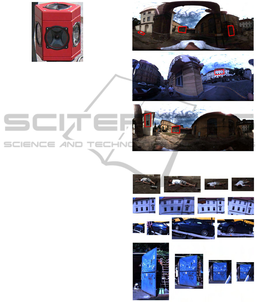
Figure 3: Ladybug 3 with 5 cameras placed horizontaly in
circle and one camera looking upwards for capturing omni-
directional images.
single image. The detector and the tracker perform
best on planar objects, because of the modeled 2D
homography transformation. We tested our algorithm
also on non-planar objects (lying human, crashed car)
to see the performance limits and robustnes of our so-
lution, see Section 3.3. Algorithm was tested on 8 ob-
jects in 4 videosequences. The ladybug camera pro-
vides 8 fps of panoramic images captured from 6 cam-
eras simultaneously. Five cameras are set horizon-
taly in a circle and the sixth camera looks upwards,
see Fig. 3. The panoramic image is a composition
of these 6 images and has resolution of 5400×2248
pixels (12 Mpx). Fig. 1 and Fig. 4 show examples
of the composed scenes and tested objects. Appear-
ance changes for few selected objects are depicted in
Fig. 5. Notice the amount of non-linear distorsion
caused by the cylindrical projection. The objects of
interest are relatively small in comparison to the im-
age size. In average the object size was 400 × 300
pixels. The ground-truth homography for each object
was manually labeled in each frame. For evaluation of
the detection/tracking performance we provide ROC
curves for each tested object. The ROC curve illus-
trates false positive rate versus false negative rate.
• False positive (FP) is a positive vote for an object
presence in some position, but the object was not
there.
• False negative (FN) is a negative vote for an ob-
ject presence in some position, where the object
actually was present.
In ROC diagrams we want to get as close to the point
(0,0) as possible. Each point in the curve of ROC
diagram is evaluated for one particular confidence
threshold c. In our system the confidence r for one
detection is given by the number of affine RANSAC
inliers after positive detection. The tracker keeps the
confidence from last detection until the loss-of-track.
With growing confidence we get less false positives,
but also more false negatives (we may miss some pos-
itive detections). For one particular c we compute the
Figure 4: Example images with tracked objects marked by
red rectangles.
Figure 5: Four of eight tested objects under different view
angles and appearances.
diagram coordinates as follows:
FP(c) =
n
∑
j=1
(F
P,where r
j
> c)/n (8)
FN(c) =
n
∑
j=1
(FN,where r
j
> c)/n, (9)
VISAPP 2011 - International Conference on Computer Vision Theory and Applications
526
where n is a number of frames in sequence. To draw
the whole ROC curve we compute the coordinates
for a discrete number of confidences from interval
< 0, 1 > and use linear interpolation for rest of the
values.
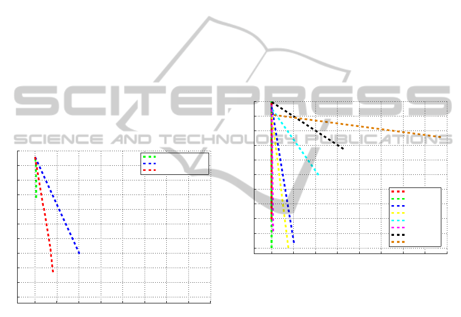
In Fig. 6 we show three different ROC curves.
Each curve corresponds to one method used to search
for the object position in sequences. In order to make
the evaluation less dependent on a particular object,
we computed mean ROC curves overall tested objects
for different methods. The green curve depicts the
performance of the tracker itself, run on every object
from the first frame until the loss-of-track without the
recoveryby the detector. The blue curve shows results
obtained by the fern detector itself run on every frame
of all sequences. And finally the red curve shows re-
sults, when our algorithm was used. We may observe,
that our algorithm performance is better (curve is the
closest to point (0,0)) than both individual methods.
The separate ROC curves for individual objects may
be seen in Fig. 7 and Fig. 9. The experiments are or-
0 0.05 0.1 0.15 0.2 0.25 0.3 0.35 0.4
0
0.1
0.2
0.3
0.4
0.5
0.6
0.7
0.8
0.9
1
COMPARISON OF METHODS
FN
FP
tracking only
detection only
detection + tracking
Figure 6: Each curve corresponds to results of one method
computed as mean ROC curve over all objects.
ganised as follows. The ferns detector is evaluated in
Section 3.1, the performance of tracker is examined in
Section 3.2. The algorithm 1, which combines both is
evaluated in Section 3.3. And finally in Section 3.4
we provide computation times of all main parts of the
algorithm.
3.1 Detector Evaluation
Using only the detector (tracking by detection) would
be too slow for desired real-time performance in se-
quence of large images. Nevertheless we evaluate the
performance of the detector itself to see how the adi-
tion of SLLiP tracker lowers the false positive and
false negative rate (see Section 3.3).
In this experiment the detector was run with
slightly different set of parameters than in the exper-
iment which combines it with the tracker. This was
necessary in order to achieve the best detection per-
formance. For example here it was not possible to
aditionally validate the positive detection by the val-
idator. So we needed to increase the threshold for
number of RANSAC inliers necessary for positive de-
tection to lower the number of false positives.
It was also necessary to adjust the detector pa-
rameters according to expected object scale and ro-
tation changes. In average the detector was search-
ing for the object in 3 scales and it was able to de-
tect objects under ±20 degrees rotation. In Fig. 7,
the ROC curves are depicted for detector run in ev-
ery frame for different objects. The results show that
0 0.05 0.1 0.15 0.2 0.25 0.3 0.35 0.4
0
0.1
0.2
0.3
0.4
0.5
0.6
0.7
0.8
0.9
1
DETECTION ONLY
FN
FP
windows
building
blue_door
wall
car
white_blocks
human
door
Figure 7: Each curve corresponds to detection results for
one object.
some objects were detected in almost all cases cor-
rectly, while some other objects, like the door, with
poor results. Door was the most complicated ob-
ject for harris corners-based detector, since only 21
keypoints were detected over the object, which were
spread mostly in the central part of the door. That
is why there was almost always a low number of in-
liers comming out of the RANSAC algorithm. This
object was lately successfuly tracked by the tracker.
Another complicated object was the car, due to its
reflective surface and vast visual angle changes. Fi-
nally, the human lying on the floor was also a chal-
lenging object due to its non-planarity. As you will
see in Section 3.3, the integration of tracking to the
algorithm lowers the number of FP and FN and sig-
nificantly speeds up the algorithm, see Section 3.4.
FAST LEARNABLE OBJECT TRACKING AND DETECTION IN HIGH-RESOLUTION OMNIDIRECTIONAL
IMAGES
527
3.2 Tracker Evaluation
This experiment shows performance of the tracker
without the recovery by the detector. The tracker is
composed of 2 SLLiPs (for translation and homog-
raphy). Each SLLiP has 3 predictors in sequence
with support set sizes |X
1
| = 225, |X
2
| = 324 and
|X
3
| = 441. The support set coordinates were spread
over the object in regular grid. The tracker was incre-
mentaly learned and validated during tracking until it
lost its track or until the end of sequence. The tracking
was manually initialized always in the first image of
sequence (different form training image), where the
object appeared. Some objects were tracked through
the whole sequence. Some objects were lost after few
frames, when there was fast motion right in the begin-
ning. In Fig. 8 you may see the lengths of successful
tracking until the first loss-of-track. In case of partial
0 50 100 150 200 250 300 350 400 450
0
1
2
3
4
5
6
7
8
9
TRACK LENGTHS
OBJECTS
FRAMES
windows
building
blue_door
wall
car
white_blocks
human
door
Figure 8: Each horizontal line depicts the length of track
for one object until the first loss-of-track. The red vertical
lines show the last frame of particular subsequence, where
the object was fully or partially visible.
occlusion the tracker sometimes jitters or even fails.
Nevertheless, when it is incrementally learned, it is
able to handle the occlusion as a new object appear-
ance. Incremental learning itself is very helpful for in-
creasing the robustness of the tracker (Hinterstoisser
et al., 2008), (Hurych and Svoboda, 2010). The esti-
mation of homography is very precise for planar ob-
jects.
Tracked objects appear in images as patches in
resolutions varying from 211× 157 (33 127 pixels) to
253 × 919 (232 507 pixels). Both SLLiPs work only
with the subset of all patch pixels (same subset size
for all objects). When tracking, each SLLiP needs
to read only 990 intensity values, which is given by
the sum of support set sizes of predictors in sequence.
This brings another significant speed-up for the learn-
ing and tracking process.
3.3 Detector + Tracker Evaluation
Final experiment evaluates the performance of algo-
rithm described in Section 2.3. The combination of
the detector and the tracker improvesthe performance
of the algorithm (lowers FP and FN), as may be seen
in Fig. 9 and Fig. 6. This is caused by their com-
plementarity in failure cases. Tracker is very robust
even under extreme perspective deformations, while
the detector is not able to recognize these difficult ob-
ject poses. On the other hand the detector is robust
to partial occlusion, where the tracker usually fails
and needs to be recovered and re-learned. In com-
0 0.05 0.1 0.15 0.2 0.25 0.3 0.35 0.4
0
0.1
0.2
0.3
0.4
0.5
0.6
0.7
0.8
0.9
1
DETECTION + TRACKING
FN
FP
windows
building
blue_door
wall
car
white_blocks
human
door
non−planar objects
planar objects
Figure 9: Each curve corresponds to results of one object
detection and tracking. The ROC curves fit more to the left
side of the diagram. This is caused by the high confidence
of detections and tracking. The high confidence is actually
valid, because of the very low number of false positives, as
we may observe.
parison with the detector (see Fig. 7), our algorithm
in average significantly improves the results. Only
few objects, which were perfectly detected by the de-
tector (e.g. white blocks and blue door) have a little
worse results with our algorithm. This was caused
by the tracking validation, which was running not ev-
ery frame, but only every 5 frames, which means, that
the tracker was lost a few frames just before loss-of-
track detection by validation and received a few FPs
and FNs. This small error could be eliminated by run-
ning the validation in every frame. The extreme effi-
ciency of sequential predictors allows tracking much
faster than real-time, which provides enough compu-
tational time for validation and incremental learning
of the tracker. Running validation after each positive
detection allows us to make the ferns detector more
VISAPP 2011 - International Conference on Computer Vision Theory and Applications
528

sensitive. We lower the threshold which specifies the
number of neccessary inliers, which allows more true
positive, but also more false positive detections. After
each detection, which has small number of inliers, we
initialize the tracker in detected pose, let the tracker
vote for homography and run the validation. Valida-
tion eliminates possible false positive detections and
let pass the true positives.
The most difficult object for our algorithm was the
crashed car, the appearance of which was changing
signifficantly during the sequence, due to its reflective
surface, non-planar shape and vast changes in visual
angle. Detection and tracking of lying human was
successful in high percentage of detected occurences
and low FP and FN. But the precision of homogra-
phy estimation was quite poor as expected, because
of its non-planar geometry. Nevertheless the incre-
mental learning kept the tracker from loosing its track
too often. The robust detector and incremental learn-
ing of the tracker allows for tracking of more complex
(non-planar) objects, but high precision homography
estimation can not be expected. Planar or semi-planar
objects were detected and tracked with high accuracy.
3.4 Computation Times
The algorithm was run on standard PC with 64 bit,
2.66 GHz CPU. The object detector was implemented
in language C and run in the system as MEX. The
RANSAC, 2-SLLiP tracker and the rest of the algo-
rithm were implemented in Matlab. When we preter-
mit the high resolution images, the PC memory re-
quirements were minimal. The computation times for
12 Mpx image sequences are following:
(implementation in language C)
• detector learning: 2 sec for 200 classes, i.e. 10 ms
per class (50 ferns with depth 11 and 500 training
samples per class).
• detection: 0.13 ms for evaluation of 1 harris point
with 50 ferns and 200 classes. The computational
time changes linearly with the number of classes.
For one image with 5350 harrises, which passed
the quality threshold, it took 0.7 sec. Usually we
run the detector in 3 scales.
(implementation in Matlab)
• learning SLLiP trackers: 6 sec for the translation
SLLiP with 1500 training samples and 9 sec for
the homography SLLiP with 3500 training sam-
ples.
• tracking: 4 ms per image. This computational
time is summed for both SLLiP trackers.
• validation: 72 ms per one validation. In our ex-
periments, the validation was run every 5 frames
during tracking.
• incremental learning: 470 ms together for 10 sam-
ples for the translation SLLiP and 10 samples for
the homography SLLiP. Incremental learning was
triggered every 5 frames after successful valida-
tion.
Average amount of harris points in one image was
around 50000, from which around 5300 passed the
harris quality threshold (Shi and Tomasi, 1994) and
were evaluated by ferns detector. The use of object
detector is neccessary, but its runtime needs to be re-
duced to a minimum because of the high computa-
tional time. The tracker runs very fast, which allows
for multiple object tracking, incremental learning and
tracking validation.
4 CONCLUSIONS AND FUTURE
WORK
In this work we combined ferns-based object detec-
tor and 2-SLLiP tracker in an efficient algorithm suit-
able for real-time processing of high resolution im-
ages. The amount of streamed data is huge and we
need to avoid running the detector too often. That
is why we focused on updating the 2-SLLiP model
during tracking, which helped to keep the track even
when the object appeared under serious slope angles
and with changing appearance. In comparison with
the detector run on every frame, our algorithm runs
not only much faster, but also lowers the number of
false positives and false negatives.
In our future work we want to focus on incre-
mental learning of both the detector and the tracker.
The detector is robust to partial occlusion, since it
works with harris corners (Harris and Stephen, 1988)
sparsely placed around the object unlike the patch-
based tracker. On the other hand the tracker is more
robust to object appearance changes and keeps track-
ing even the signifficantly distorted objects, which the
detector fails to detect. This gives the opportunity to
deliver the training examples for the detector in cases
where it fails, while the tracker holds and vice-versa.
We would like to develop a suitable strategy for mu-
tual incremental learning.
ACKNOWLEDGEMENTS
The 1st author was supported by Czech Science
Foundation Project P103/10/1585. The 2nd author
FAST LEARNABLE OBJECT TRACKING AND DETECTION IN HIGH-RESOLUTION OMNIDIRECTIONAL
IMAGES
529

was supported by Czech Science Foundation Project
P103/11/P700. The 3rd author was supported by EC
project FP7-ICT-247870 NIFTi. Any opinions ex-
pressed in this paper do not necessarily reflect the
views of the European Community. The Community
is not liable for any use that may be made of the in-
formation contained herein.
REFERENCES
Baker, S. and Matthews, I. (2004). Lucas-kanade 20 years
on: A unifying framework. In International Journal
of Computer Vision, volume 56, pages 221–255.
Bay, H., Ess, A., Tuytelaars, T., and Van Gool, L. (2006).
Speeded-up robust features. In Proceedings of IEEE
European Conference on Computer Vision, pages
404–417.
Dellaert, F. and Collins, R. (1999). Fast image-based track-
ing by selective pixel integration. In Proceedings
of the International Conference on Computer Vision:
Workshop of Frame-Rate Vision, pages 1–22.
Hager, G. D. and Belhumeur, P. N. (1998). Efficient region
tracking with parametric models of geometry and illu-
mination. IEEE Transactions on Pattern Analysis and
Machine Intelligence, 20(10):1025–1039.
Harris, C. and Stephen, M. (1988). A combined corner
and edge detection. In Matthews, M. M., editor, Pro-
ceedings of the 4th ALVEY vision conference, pages
147–151, University of Manchaster, England. on-line
copies available on the web.
Hinterstoisser, S., Benhimane, S., Navab, N., Fua, P., and
Lepetit, V. (2008). Online learning of patch perspec-
tive rectification for efficient object detection. In Con-
ference on Computer Vision and Pattern Recognition,
pages 1–8.
Holzer, S., Ilic, S., and Navab, N. (2010). Adaptive lin-
ear predictors for real-time tracking. In Conference
on Computer Vision and Pattern Recognition (CVPR),
2010 IEEE, pages 1807–1814.
Hurych, D. and Svoboda, T. (2010). Incremental learn-
ing and validation of sequential predictors in video
browsing application. In VISIGRAPP 2010: Inter-
national Joint Conference on Computer Vision, Imag-
ing and Computer Graphics Theory and Applications,
volume 1, pages 467–474.
Jurie, F. and Dhome, M. (2002). Hyperplane approximation
for template matching. IEEE Transactions on Pattern
Analysis and Machine Intelligence, 24:996–1000.
Li, M., Chen, W., Huang, K., and Tan, T. (2010). Vi-
sual tracking via incremental self-tuning particle fil-
tering on the affine group. In Conference on Computer
Vision and Pattern Recognition (CVPR), 2010 IEEE,
pages 1315–1322.
Lowe, D. (2004). Distinctive image features from scale-
invariant keypoints. International Journal on Com-
puter Vision, 60(2):91–110.
Lucas, B. and Kanade, T. (1981). An iterative image regis-
tration technique with an application in stereo vision.
In Proceedings of the 7th International Conference on
Artificial Intelligence, pages 674–679.
¨
Ozuysal, M., Calonder, M., Lepetit, V., and Fua, P. (2010).
Fast keypoint recognition using random ferns. IEEE
Transactions on Pattern Analysis and Machine Intel-
ligence, 32(3):448–461.
Shi, J. and Tomasi, C. (1994). Good features to track. In
Proceedings of IEEE Computer Society Conference
on Computer Vision and Pattern Recognition, pages
593–600.
ˇ
Sochman, J. and Matas, J. (2005). Waldboost - learning
for time constrained sequential detection. In Proceed-
ings of the Conference on Computer Vision and Pat-
tern Recognition, pages 150–157.
Zimmermann, K., Matas, J., and Svoboda, T. (2009a).
Tracking by an optimal sequence of linear predictors.
IEEE Transactions on Pattern Analysis and Machine
Intelligence, 31(4):677–692.
Zimmermann, K., Svoboda, T., and Matas, J. (2009b). Any-
time learning for the NoSLLiP tracker. Image and
Vision Computing, Special Issue: Perception Action
Learning, 27(11):1695–1701.
VISAPP 2011 - International Conference on Computer Vision Theory and Applications
530
