EFFICIENT ANALYTICAL INTEGRATION OF SINGLE
SCATTERING FUNCTION
Umashankar Pradhan and Subodh Kumar
Dept. of Computer Sc. & Engg., IIT Delhi, New Delhi, India
Keywords:
Global Illumination, Scattering, Participative Media, Real time rendering.
Abstract:
Light scattering through a participative medium has a significant impact on display. However, accurate and
efficient simulation of scattering remains challenging. Monte Carlo or numerical integration techniques are
commonly employed to solve the scattering equation. Single scattering is a common approximation that
provides satisfactory results in many cases. Analytical integration of scattering under certain assumptions have
been achieved by pre-computing a table of values. We present a new approximation to the single scattering
equation that is easily integrable in real time. We analyze the error of this approximation and show that the
numerical error is insignificant. The images are virtually indistinguishable from those obtained by the more
accurate integration.
1 INTRODUCTION
Models of scattering are employed in computer
graphics for accurate display of phenomena from fog,
smoke, snow and cloud to hair, marble and skin. Op-
tical scattering refers to deviation of light from the
straight path due to particles in the medium as well
as to deviation from the specular direction after re-
flection. Scattering is important for realistic display.
Indeed, most uncontrolled environments exhibit suffi-
cient scattering to induce glows around light source
or to somewhat blur appearance of objects. Light
shafts and haziness, for example, are effects of scat-
tering common in photographs but often missing from
computer generated imagery because they are com-
plex and slow to compute.
In this paper we focus on light scattering when
traveling through participative media. We assume
particles are significantly larger than light’s wave-
length, focussing on geometric scattering. Usually
light scatters multiple times as it encounters particles
in its path. However, often single scattering approx-
imations are used, which accurately describe sparse
media – but are often useful for dense media as well.
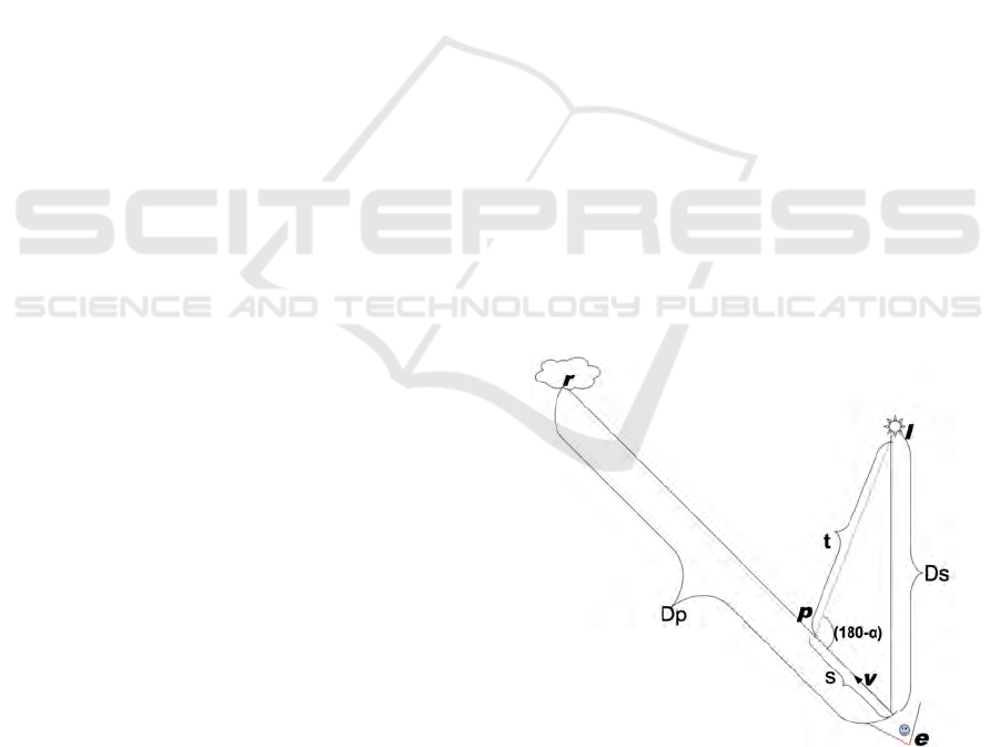
Generic single scattering is described in Figure 1.
Light from source l is scattered by a particle at p. A
fraction scatters towards viewpoint e. Such scatter-
ing takes place from all points along any direction of
view v. We integrate these to obtain the total scat-
tered radiance. This is often referred to as the airlight
Figure 1: Standard formulation of single scattring.
integral. The total radiance also includes any source
(including reflective surface) in the direction of view.
Some of this also scatters away and does not reach
the viewpoint. The radiance scattering straight ahead
is separately integrated.
Integration of the airlight function can be per-
formed by numerical techniques. However, when an-
alytical integration is possible, images can be gener-
ated significantly faster. Ours is an attempt belonging
to this genre. We approximate the scattering function
by analytically integrable ones and show that the error
is small, quantitatively as well as qualitatively.
193
Pradhan U. and Kumar S..
EFFICIENT ANALYTICAL INTEGRATION OF SINGLE SCATTERING FUNCTION.
DOI: 10.5220/0003373901930199
In Proceedings of the International Conference on Computer Graphics Theory and Applications (GRAPP-2011), pages 193-199
ISBN: 978-989-8425-45-4
Copyright
c
2011 SCITEPRESS (Science and Technology Publications, Lda.)

2 RELATED WORK
Importance of scattering has been recognized long
in computer graphics (Blinn, 1982). Even analyti-
cal models were described early (Max, 1986; Nishita
et al., 1987). Light transport equations (Chan-
drasekhar, 1960) are often solved using Monte Carlo
techniques (Stam, 1994; Lafortune, 1996; Jensen and
Christensen, 1998) and finite element method (Rush-
meier and Torrance, 1987; Sillion, 1994; Arbree et al.,
2010a; Arbree et al., 2010b). Both are expensive.
(Premoze et al., 2004) use point spread func-
tions to compute airlight due to multiple scattering.
(Sun and Ramamoorthi, 2005) attempt to perform the
airlight integral analytically and our work is inspired
by theirs. The integral however does not admit ana-
lytical solution. (Sun and Ramamoorthi, 2005) hence
precompute a 2D table, assuming that the medium
density and scattering coefficients are known. The in-
termediate values are then evaluated using interpola-
tion. We, instead, derive functions that track the in-
tegral for different values of medium density and par-
ticle sizes. And, we do not require precomputation
at a pre-determined resolution. Further, we incorpo-
rate backward scattering as well. Our work is also
similar in spirit to that of (Biri et al., 2006) who use
a polynomials of degree four to approximate the ker-
nel. However, the function is not well approximated
by polynomials and their approximation incurs unac-
ceptably large error (as shown later).
Later (Zhou et al., 2007) provide an analytic ap-
proximation to the airlight integral in the presence
of inhomogeneous media whose density can be de-
scribed as a sum of Gaussians. The airlight integral is
performed for each Gaussian. More recently (Bern-
abei et al., 2010) propose a spherical harmonics based
representation of inhomogeneous material properties.
They subdivide inhomogenous media into voxels and
sample for each voxel, the attenuation of light in var-
ious directions. Spherical harmonics based represen-
tation of these samples is used to later integrate along
a ray. In the next sections we describe our approxima-
tion and present error analysis and rendering results.
3 SINGLE SCATTERING
INTEGRAL
This table lists the terminology for reference (see
also Figure 1):
I
s
= Radiant intensity of the point light
source
D
s
= Distance of the light source from the in-
tegration point (view point)
θ
s
= Angle between the direction of integra-
tion and the direction to light
α = Phase angle of scattering
P(α) = Phase function for anisotropic scattering
x = Distance of the scattering point from the
perpendicular to light source (forward
scattering)
t
x
= Distance of the light source from the
point of forward scattering
y = Distance of the scattering point from the
perpendicular to light source (backward
scattering)
t
y
= Distance of the light source from the
point of backward scattering
The radiance L comprises the direct transmission
component L
d
and the single scattering radiance
(airlight), L
a
: L = L
d
+ L
a
. The direct term L
d
simply
attenuates the incident radiance from a point source
by an exponential corresponding to the distance be-
tween the source and the viewer and the scattering
coefficient β:
L
d
(θ
s
, D
s
, β) =
I
s
D
2
s
e
−βD
s
δ(θ
s
),
where the impulse function δ indicates that the direct
component is non-zero only in the direction of the
light (i.e., point light source or reflective point on a
surface). The airlight component (Nishita et al., 1987)
is:
L
a
(θ
s
, D
s
, D
p
, β) =
Z
D
p
0
βP(α)
I
s
e
−βt
t
2
e
−βs
ds,
Figure 2: Forward Scattering.
where D
p
is the distance to the closest surface
point along the view direction, or ∞ if no such sur-
face exists. The integration is over single scattering at
GRAPP 2011 - International Conference on Computer Graphics Theory and Applications
194
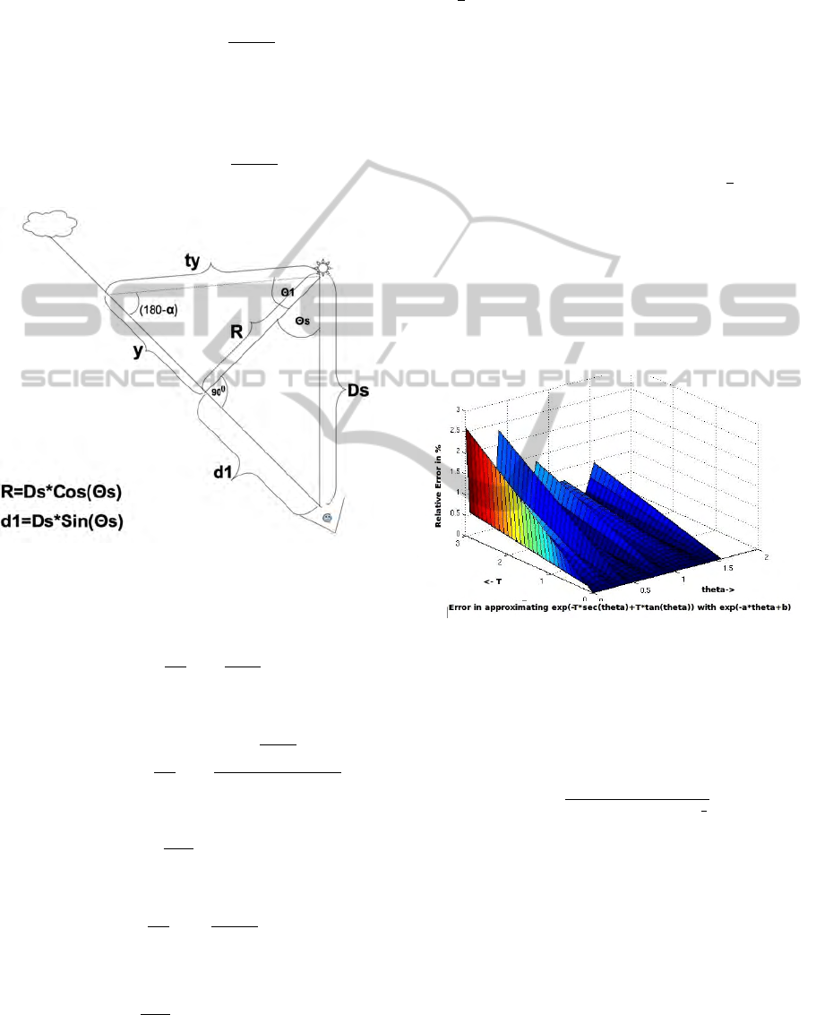
distance s from the viewer and t is the distance of the
scattering point from the source of light. Subdividing
the integral into parts L
1
(forward scattering) and L
2
(backward scattering):
L
1
(θ
s
, D
s
, D
p
, β) =
Z
d
1
0
βP(α)
I
s
e
−βt
x
t
2
x
e
−β(d
1
−x)
dx,
where d
1
= D
s
sinθ
s
. Figure 2 illustrates the case
when the scattering angle α is less than 90
◦
and Fig-
ure 3 does when the angle is more than 90
◦
.
L
2
(θ
s
, D
s
, D
p
, β) =
Z
D
p
0
βP(α)
I
s
e
−βt
y
t
2
y
e
−β(y+d
1
)
dy.
Figure 3: Backward Scattering.
Consider L
1
first, with the default isotropic phase
function:
L
1
(θ
s
, D
s
, D
p
, β) =
βI
s
4π
Z
d
1
0
e
−βt
x
t
2
x
e
−β(d
1
−x)
dx,
with t
2
x
= x
2
+ R
2
(and R = D
s
cosθ
s
). Thus:
L
1
(θ
s
, D
s
, D
p
, β) =
βI
s
4π
Z
d
1
0
e
−β(
√
x
2
+R
2
+d
1
−x)
t
2
x
dx
With x = R tanθ:
L
1
(θ
s
, D
s
, D
p
, β) =
βI
s
4πR
Z
θ
s
0
e
−βR(secθ−tanθ)
dθ
Similarly,
L
2
(θ
s
, D
s
, D
p
, β) =
I
s
β
4π
Z
D
p
0
I
s
e
−βt
y
t
2
y
e
−β(y+d
1
)
dy. (1)
And with t
2
y
= R
2
+ y
2
and y = Rtanθ,
L
2
(θ
s
, D
s
, D
p
, β) =
I
s
β
4πR
e
−βd
1
Z
θ
1
0
e
−βR(secθ+tanθ)
dθ,
(2)
where θ
1
is the angle made by the vector from the
light to surface and the perpendicular to the direction
of view as shown in Figure 3. If there is no surface,
θ
1
is
π
2
.
3.1 Forward Scattering Approximation
In order to compute the integrals in equations 1 and 2,
we use the following approximation to sec θ −tan θ ≈
−0.8405θ + 0.9915, 0 ≤θ ≤ 0.3959
−0.6331θ + 0.9094, 0.3959 ≤θ ≤ 0.8395
−0.5216θ + 0.8158, 0.8395 ≤θ ≤
π
2
This is a low error piecewise linear approximation
to secθ −tanθ. Now this function can by analytically
integrated. The error is less than the precomputed ta-
ble of (Sun and Ramamoorthi, 2005) once the entire
integral is evaluated. Figure 4 shows the relative er-
ror in our approximation. As a comparison, the poly-
nomial based error (Biri et al., 2006) is many times
higher as shown in Figure 5
Figure 4: Relative error in overall radiance due to the
secθ −tan θ approximation.(T = βR).
Although isotropic scattering phase function
is commonly used in many implementations, the
Henyey Greenstein phase function approximation
(Henyey and Greenstein, 1941):
P(α) =
1 −g
2
(1 + g
2
−2g cos α)
3
2
produces more realistic results. Here g is usually
taken as a constant property of the medium. This
can be incorporated into our system again by using
a Gaussian like form: P(x) ≈ae
−bx
where a and b are
quadratic functions of g:
a = a
1
g
2
+ a
2
g + a
3
b = b
1
g
2
+ b
2
g + b
3
Now a
i
and b
i
are chosen to provide the best fit,
still ensuring a small error. For the error to remain
EFFICIENT ANALYTICAL INTEGRATION OF SINGLE SCATTERING FUNCTION
195
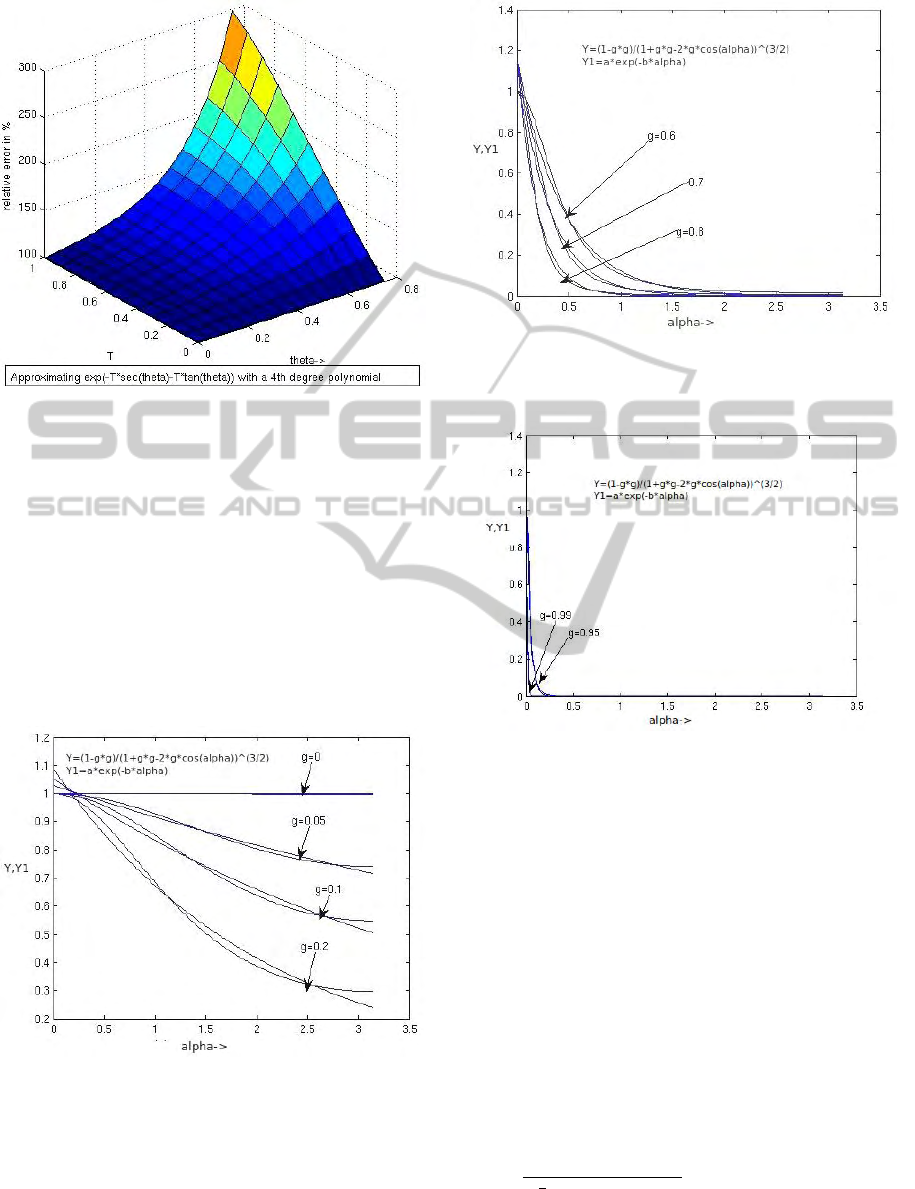
Figure 5: Relative error in radiance due to polynomial ap-
proximation (Biri et al., 2006).(compare to Figure 4.)
bounded, different a
i
and b
i
values are needed for dif-
ferent ranges of g. The detailed set of coefficients,
which generate low error, are reproduced in the ap-
pendix. Note that the value of g will be constant for
a uniform medium and known at the rendering time
and hence only one of these will be used. We show
here the error for a few values of g. Recall that g lies
between 0 and 1, g near 0 for little scattering and g
near 1 for denser media like haze and fog. The max-
imal error we observe is for lower values of g and it
reduces as g increases.
Figure 6: Comparing our approximation to the Henyeye
Greenstein approximation for increasing values of phase an-
gle α: 0 ≤ g ≤ 0.2. The original and our approximation
curves are shown. The maximum error is for this range of
g and occurs near α = 0. Values of g less than 0.5 are not
commonly used.
Figure 7: Comparing our approximation to the Henyeye
Greenstein approximation for increasing values of phase an-
gle α: 0.6 ≤ g ≤ 0.8.
Figure 8: Comparing our approximation to the Henyeye
Greenstein approximation for increasing values of phase an-
gle α: 0.95 ≤ g ≤ 0.99.
3.2 Backward Scattering
Approximation
Although the backward scattering component is usu-
ally much smaller than the forward scattering compo-
nent, we include this as well for completeness. Unfor-
tunately, however, a simple low-error approximation
to the kernel for L
2
seems harder to find. Instead we
are able to better approximate the ratio between the
forward and the backward parts of the integral. Ob-
serving the nature of the resulting ratio, we approxi-
mate it with the following exponential:
R
θ
1
0
e
−κ(secθ+tanθ)
dθ
R
π
2
0
e
−κ(secθ−tanθ)
dθ
= f (θ
1
)e
−g(θ
1
)κ
h(θ
1
)
where,
GRAPP 2011 - International Conference on Computer Graphics Theory and Applications
196
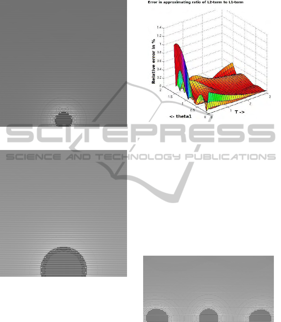
Figure 9: Rendered airlight using Henyeye Greenstein
phase function with g=0.7 and β = 0.05.
Figure 10: Rendered airlight using Henyeye Greenstein
phase function with g=0.4 and β = 0.05.
f (θ
1
)
g(θ
1
)
h(θ
1
)
=
−0.0394 0.1065 0.5774 0.0058
−0.1299 0.4204 0.3811 0.5993
0.0171 −0.1586 −0.0424 1.0879
θ
3
1
θ
2
1
θ
1
1
Achieving quantitatively small fractional error for
backward scattering with Henyey GreenStein phase
function remains an open problem. However, since
the magnitude of this component is usually smaller,
even large fractional error does not produce notice-
able differences in the final image. The error graph is
shown in Figure 11.
Figure 11: The error in the radiance due to the back-scatter
approximation by relating the integral to the forward-
scattering.
4 EXPERIMENTS AND RESULTS
We have implemented our approximations on an Intel
Centrino based linux laptop PC with 4GB RAM and
an nVIDIA GT-240M graphics processor. We imple-
mented the integration in the pixel shader and are able
to render scenes such as shown in Figure 18 more than
90 times a second on a 512x512 pixel screen. The il-
lumination behavior is as expected. As the value of
the extinction coefficient β becomes smaller, the glow
size decreases (Figures 12 and 13). Also, the glow
sizes of distant light is smaller than the one closer
(Figure 14).
Figure 12: Rendered using pixel shader. β = 0.01. Lower β
implies smaller glows.
Figures 15 shows an example demonstrating that
backward scattering has a small effect on the images.
We compare our rendering of the airlight to a
povRay based implementation of Monte Carlo inte-
gration in Figure 16. We use the intensity distribution
of the glow to demnstrate the difference because full
EFFICIENT ANALYTICAL INTEGRATION OF SINGLE SCATTERING FUNCTION
197
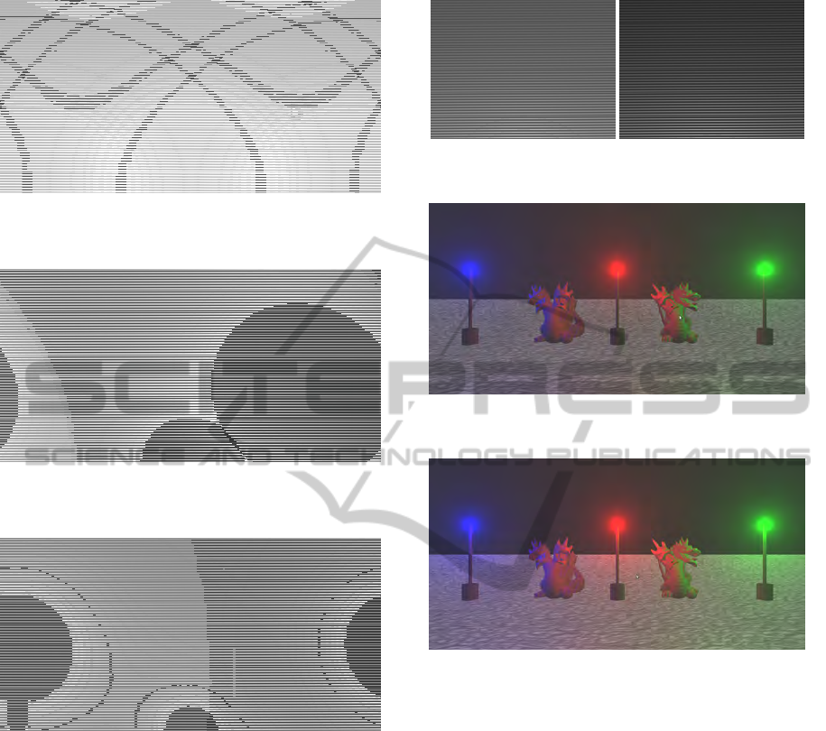
Figure 13: Rendered using pixel shader. β = 0.04. As β
increases, glow does too.
Figure 14: Rendered using pixel shader. β = 0.04. Far away
light has less glow.
Figure 15: Rendered using pixel shader. Forward scattering
only β = 0.04.
scene renderings tend to hide differences. Although
the differences are noticeable, the overall qualitative
structures of the scenes are comparable. As a point of
reference, the povRay implementation takes 10 sec-
onds to render this scene while our pixel shader based
implementation renders the same scene more than a
thousand times a second.
5 CONCLUSIONS
Out goal was to find an accurate and efficient approx-
imation for the single scattering integral. As a re-
sult of this, the entire integral can be re-evaluated at
each pixel at interactive rates. Since there is no pre-
Figure 16: Comparison of our rendering (left) with
povRay’s (using istropic phase function).
Figure 17: A scene with a dragon model rendered without
surface scattering.
Figure 18: A scene with a dragon model rendered with sur-
face scattering. The dragons consist of more than 100,000
triangles.
computation, changes to the particle density, for ex-
ample due to increasing rain, can be easily handled.
We have not focussed on surface scattering effects
or shadows, which can easily be incorporated follow-
ing (Sun and Ramamoorthi, 2005) and (Biri et al.,
2006). For example, we demonstrate surface scatter-
ing effect in Figures 17 and 18. The errors introduced
by our approximations are quite low and we feel the
derived coefficient would be useful to many others. At
the same time, even with an unoptimized code render-
ing is fast.
REFERENCES
Arbree, A., Walter, B., and Bala, K. (2010a). Heteroge-
neous subsurface scattering using the finite element
method. IEEE Transactions on Visualization and
Computer Graphics, 99(PrePrints).
GRAPP 2011 - International Conference on Computer Graphics Theory and Applications
198

Arbree, A., Walter, B., and Bala, K. (2010b). Heteroge-
neous subsurface scattering using the finite element
method. IEEE Transactions on Visualization and
Computer Graphics, 99(PrePrints).
Bernabei, D., Ganovelli, F., Pietroni, N., Cignoni, P., Pat-
tanaik, S., and Scopigno, R. (2010). Real-time single
scattering inside inhomogeneous materials. Vis. Com-
put., 26(6-8):583–593.
Biri, V., Michelin, S., and Arques, D. (2006). Real time ren-
dering of atmospheric scattering and volumetric shad-
ows. In Journal of WSGC, pages 65–72.
Blinn, J. F. (1982). Light reflection functions for simula-
tion of clouds and dusty surfaces. In Proceedings of
the 9th annual conference on Computer graphics and
interactive techniques, SIGGRAPH ’82, pages 21–29,
New York, NY, USA. ACM.
Cerezo, E., Perez, F., Pueyo, X., Seron, F. J., and Sillion,
F. X. (2005). A survey on participating media render-
ing techniques. The Visual Computer, 21(5):303–328.
Chandrasekhar, S. (1960). Radiative Transfer. Dover Pub-
lications.
Henyey, L. and Greenstein, J. (1941). Diffuse radiation in
the galaxy. Astrophys. Journal, 93:70–83.
Jensen, H. W. and Christensen, P. H. (1998). Efficient sim-
ulation of light transport in scences with participating
media using photon maps. In Proceedings of the 25th
annual conference on Computer graphics and inter-
active techniques, SIGGRAPH ’98, pages 311–320,
New York, NY, USA. ACM.
Lafortune, E. (1996). Mathematical Models and Monte
Carlo Algorithms for Physically Based Rendering.
PhD thesis, Cornell University.
Max, N. L. (1986). Atmospheric illumination and shad-
ows. In Proceedings of the 13th annual conference on
Computer graphics and interactive techniques, SIG-
GRAPH ’86, pages 117–124, New York, NY, USA.
ACM.
Nishita, T., Miyawaki, Y., and Nakamae, E. (1987). A shad-
ing model for atmospheric scattering considering lu-
minous intensity distribution of light sources. SIG-
GRAPH Comput. Graph., 21:303–310.
Premoze, S., Ashikhmin, M., Ramamoorthi, R., and Nayar,
S. K. (2004). Practical rendering of multiple scatter-
ing effects in participating media. In Rendering Tech-
niques, pages 363–373.
Rushmeier, H. E. and Torrance, K. E. (1987). The zonal
method for calculating light intensities in the pres-
ence of a participating medium. SIGGRAPH Comput.
Graph., 21:293–302.
Sillion, F. (1994). Clustering and volume scattering for hier-
archical radiosity calculations. In In Fifth Eurograph-
ics Workshop on Rendering, pages 105–117.
Stam, J. (1994). Stochastic rendering of density fields. In
Proceedings of Graphics Interface 94, pages 51–58.
Sun, B. and Ramamoorthi, R. (2005). A practical analytic
single scattering model for real time rendering. ACM
Trans. Graph, 24:1040–1049.
Zhou, K., Hou, Q., Gong, M., Snyder, J., Guo, B., and
Shum, H.-Y. (2007). Fogshop: Real-time design and
rendering of inhomogeneous, single-scattering me-
dia. In Proceedings of the 15th Pacific Conference
on Computer Graphics and Applications, pages 116–
125, Washington, DC, USA. IEEE Computer Society.
APPENDIX
Phase Function Approximation
The matrix below are in the format:
a
1
a
2
a
3
b
1
b
2
b
3
If 0 ≤ g ≤ 0.2 :
−0.8470 0.6117 1.0004
0.7218 2.2603 0.0009
If 0.2 ≤ g ≤ 0.4 :
−0.3199 0.4128 1.0197
3.1063 1.2475 0.1109
If 0.4 ≤ g ≤ 0.6 :
−0.2697 0.3865 1.0223
9.4069 −4.0092 1.2134
If 0.6 ≤g ≤ 0.8 :
−0.3067 0.4298 1.0096
46.9285 −51.3639 16.1729
If 0.8 ≤g ≤ 0.9 :
−1.1784 1.8440 0.4358
369.6793 −573.3485 227.3450
If 0.9 ≤ g ≤ 0.95 :
−7.5 13.3 −4.7
2829.9 −5022.1 2238.6
If 0.95 ≤ g ≤ 0.99 :
−50 90 −40
78630 −150550 72090
EFFICIENT ANALYTICAL INTEGRATION OF SINGLE SCATTERING FUNCTION
199
