TWO-LEVEL STRATEGY

FOR IMAGE BOUNDARY DETECTION

Karin S. Komati, Evandro O. T. Salles and Mario Sarcinelli-Filho

Graduate Program on Electrical Engineering, UFES, Av. Fernando Ferrari, 514, Vitória/ES, Brazil

Keywords: Boundary detection, Multifractal measurement, J value, 1/f spectrum, Region-growing, Edge detection.

Abstract: A new method for boundary detection in natural images is here proposed, consisting of two levels, or two-

stage sequential processes: embedded integration and post-processing integration. In the embedded

integration, two different methods to measure homogeneity in region-growing technique are integrated,

based on a global statistical property: the shape of the power spectrum of the image being analyzed. One

homogeneity measure is the J value (provided by the classical JSEG algorithm) and the second measure is a

multifractal measurement. This first step provides a region extraction. In the second level, edge information

is extracted by a classical method, and integrated with region information. This structure, called KSS,

eliminates false boundaries in the region map, guided by the edge map, and the noise in edge map as well,

now guided by the region map, thus taking the advantage of their complementary nature. Experiments on a

large dataset of natural color images show that the result of such two-level strategy matches the human

perception better than the individual methods, quantitatively and qualitatively speaking.

1 INTRODUCTION

Boundary detection is one of the most important

tasks in computer vision. Traditionally, the

techniques can be classified in region or edge

approaches. There may exist gaps and noisy edges in

edge-approach results, whereas region-approach

results tend to be over-segmented with inaccurate

boundaries. There are many proposals combining the

outputs of region-growing and edge detection

methods to improve the quality of their results.

Muñoz, Freixenet, Cufí and Martí (2003) show

seven different strategies for combining similarity

(region) and discontinuity (edge) information. They

were grouped in two classes: embedded integration

and post-processing integration.

In this work, these two classes are considered in

two sequential levels. In the embedded integration,

the J value obtained by using the classical JSEG

method (Deng and Manjunath, 2001) and a

multifractal measurement are integrated, the

integration being controlled by the shape of the

power spectrum of the image under analysis. Such

statistical property is also used to calibrate the

threshold of the merging process. The segmentation

obtained by merging the results of both individual

methods (hereinafter referred to as MM-Frac

method) is more informative than the result of each

individual method, as it is shown ahead.

Till now, the region-growing result of MM-Frac

and edge information are extracted parallely and

separately. Our strategy is to put the two maps

together, eliminating the false boundaries in the

region map, based on edge information, and

eliminating the noisy edges in the edge map, based

on region information. Such method is hereinafter

referred to as KSS (Komati, Salles and Sarcinelli-

Filho, in press). In the sequel, we show that the

resulting image is closer to human perception than

any of the two images used as input for the post-

processing integration.

Quantitative performance comparison requires

ground truth and well defined metrics. Both

requirements can be found in “The Berkeley

Segmentation Dataset and Benchmark” (BSDS)

(Martin, Fowlkes, Tal and Malik, 2001). For each

image in the BSDS, there are at least five hand-

labeled segmentations made by human beings,

which constitute the ground truth. The standard

metrics of BSDS are precision, recall and F-

measure, determining how well the boundary map

approximates the human ground truth boundaries

(Martin, Fowlkes, and Malik, 2004).

181

Komati K., Salles E. and Sarcinelli-Filho M..

TWO-LEVEL STRATEGY FOR IMAGE BOUNDARY DETECTION .

DOI: 10.5220/0003375801810186

In Proceedings of the International Conference on Computer Vision Theory and Applications (VISAPP-2011), pages 181-186

ISBN: 978-989-8425-47-8

 2011 SCITEPRESS (Science and Technology Publications, Lda.)

2 THE PROPOSED METHOD

2.1 First-Level of Integration

2.1.1 J value

The essence of the JSEG method is to separate the

segmentation process in two independently

processed stages: color quantization and spatial

segmentation. The result of color quantization is a

class-map which associates a color class label to

each pixel belonging to a class.

In the spatial segmentation stage, a criterion to

measure the distribution of color classes, the J

measure, is calculated. Essentially, it measures the

distances between different classes, divided by the

distances between the members within each class, an

idea similar to the Fisher's multi-class linear

discriminator. The J value can be calculated by

using a local area of the class-map. Multi-scale J-

images are calculated changing the local window

size. In the J-image, the higher the local J value is,

the more likely the pixel is part of a boundary

region, like a 3-D terrain map containing valleys and

mountains. Then, a region growing method is used

to segment the image. Finally, to overcome the over-

segmentation problem, regions are merged based on

their color similarities, by directly applying a

Euclidean distance measure.

2.1.2 The Multifractal Measurement

In this work, we will use the differential box-

counting method, proposed by Chaudhuri and Sarkar

(1995), to estimate the multifractal measurement

(MM) of the original image.

The MM of a single pixel is calculated in a small

window surrounding it, generating a Fractal-image

for each channel in Luv color space (Komati et al.,

2010). The Fractal-images are also a 3D terrain

maps, that is because the MM in the border regions

of a texture is lower than the MM of a homogeneous

region (Pentland, 1984). Each value in Fractal-image

is converted to be higher in boundary regions and to

have the same limits applied to a J-image.

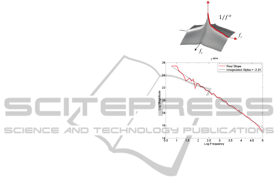
2.1.3 1/f Spectra of Natural Images

Statistics of natural images have been found to

follow particular regularities. Torralba and Oliva

(2003), studying the statistics of real-world images,

observed that the energy spectra of such images

falls, in average, into a form 1/f

with α∼2. They

also show that the shape of the power spectrum can

be used to categorize the different semantic of

scenes (single objects, rooms, places, large outdoors

and panoramic scenes).

(a)

(b)

Figure 1: Graphic of one image power spectrum (a) 3D (b)

2D.

Here α represents the slope of the decreasing

energy spectrum values, from low to high spatial

frequencies, varying with the scene complexity.

Figure 1(a) exemplifies a 3D power spectrum, where

the slope is emphasized in red. Figure 1(b) shows

the slope (red) in a 2D graphic and the interpolated

slope (the dotted black line). The estimated -α value

is then -2.31, or α value is then +2.31.

Pentland (1984) showed that fractal natural

surfaces (as mountains, forests) produce a fractal

image with an energy spectrum of the form 1/ f

where α is related to the fractal dimension of the 3D

surface (e.g., its roughness). Slope characteristics

may be grouped in two main families, a slow slope

(α∼1), for environments with textured and detailed

objects, and a steep slope (α∼3), for scenes with

large objects and smooth edges. Thus, the slower the

slope is, the more textured the image is.

2.1.4 MM-Frac

In this new proposal, the integration of two

measurements, J-image and Fractal-image, is

controlled by the value of α as in the work of Côco,

Salles, Sarcinelli-Filho (2009). Figure 2 shows a

simplified architecture of the proposed MM-Frac

VISAPP 2011 - International Conference on Computer Vision Theory and Applications

182

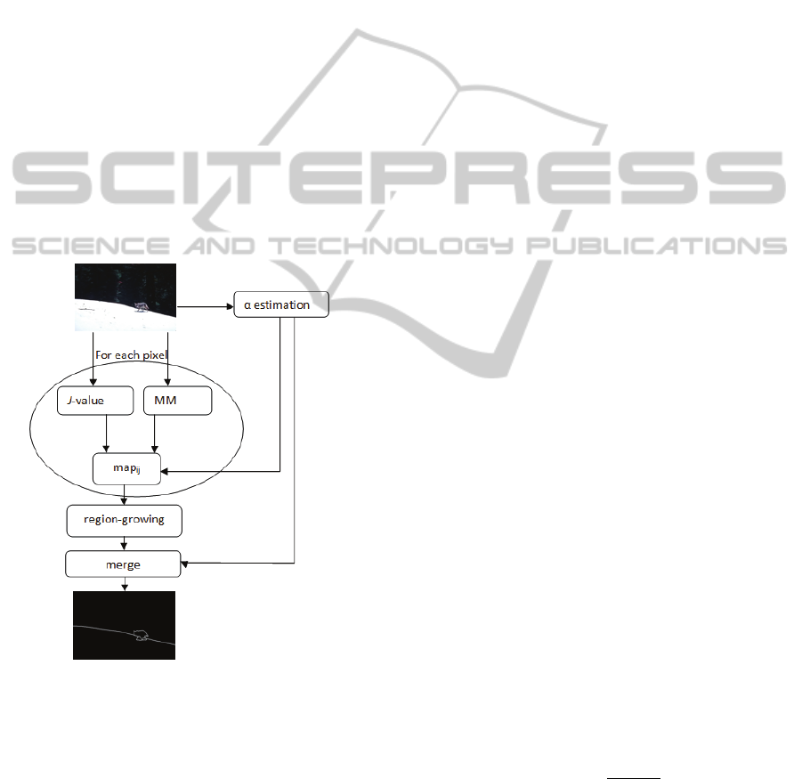
system. The global estimated value α controls two

process:

1) the local integration of the J-value and local

Fractal-value. Each pixel of the 3D terrain map is

now calculated as:

map

= J-value×α

norm

+ (1-α

norm

)×Fractal-value, (1)

where α

norm

= α/max(α

), i indexing the 200 images

used as training set (provided by BSDS). For low α

values, the image presents more texture, and the

multifractal weight is greater than that of the J-

value, as multifractal models textures in a better way

than the J-value;

2) the threshold used in region merging is

(0.4×α

norm

), where 0.4 is the default value for the

JSEG method. The lower the threshold is, lesser

regions will be merged, and the segmentation result

will present more regions with a lower threshold,

compared to a higher threshold. An image with high

α value presents large objects and smooth edges, so

it is expected that the segmentation result will

present just a few regions.

Figure 2: Simplified architecture of MM-Frac.

2.2 Second-Level of Integration

2.2.1 Edge Detection

We considered here some classical edge detectors

(Sobel, Prewitt, Laplacian and morphological

gradient), which generates an output known as a soft

boundary map, with each pixel valued from zero to

one, where higher values mean greater confidence in

the existence of a boundary. To choose a good edge

detector, it was made a preliminary test and the

morphological gradient presents the overall F-

measure slightly better than the other detectors.

Therefore, it was chosen as the edge detection

method.

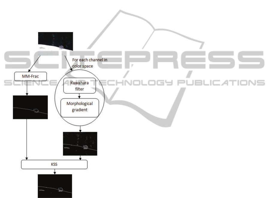
It is quite usual to smooth the image to eliminate

noise before the edge detection. We choose a

classical non-linear edge-preserving-smoothing

filter, the Kuwahara filter with 5×5 mask size. To

process a color image, each of three color channels,

RGB, is processed separately, and then all results are

added into one image.

2.2.2 Second-level of Integration: KSS

The integration method is independent of how the

edge-map and region-map are processed. However,

it is necessary that the region-map be a binary image

and the edge-map be a soft map. Figure 3 shows a

simplified architecture of the proposed KSS system.

First, we will present the algorithm as a pseudocode:

1. Inputs: edge-map and region-map

2. Set image-result as the sum of edge-map and region-

map

3. Build a weak-edge-map from edge-map

4. For each pixel

I. If (the pixel is marked as edge on region-map

and the pixel is marked as a weak on weak-edge-

map and the majority of neighborhood is marked as

a weak on weak-edge-map).

Then set non-edge in the pixel location in the

resulting image.

II. If (the pixel is marked as a non-edge on

region-map and the pixel is marked as a weak on

weak-edge-map).

Then set non-edge in the pixel location in the

resulting image.

In the step-2, the sum operation will enhance all

boundary pixels that match in the two different input

maps. In the rest of the code, the logic is to eliminate

or reduce false information. In the step-3,the purpose

is to detect the weak edges from the edge-map. To

automate the threshold value, it was used an idea

similar to the one in Rotem, Greenspan and

Goldberger (2007), the value of the threshold is

based on edge-map histogram h, and is given by

ℎℎ



∑

ℎ







∑

ℎ









(2)

where i=[0,255] is the value of a pixel in the image.

A noisy edge-map will result in low values of

threshold

weak

while a strongly defined edge-map will

result in higher values. Step-4.I eliminates false

boundaries provided by region-map and step-4.II

TWO-LEVEL STRATEGY FOR IMAGE BOUNDARY DETECTION

183

eliminates the noisy information provided by the

edge-map source. The neighbourhood of KSS weak-

edge-map was set to 3×3 for all images.

The higher the threshold

weak

value is, more weak-

edges are obtained, and thus more information will

be eliminated in the process. The result presents less

edge information in the region-map and less weak

information in the edge-map. The result seems

cleaner, preserving only the strong edges of both

maps. However, when the image is noisy, all

information about both maps is preserved, with the

strong edges emphasized. In such images, we notice

that region-map information is more valuable than

edge-map information.

Figure 3: Simplified architecture of KSS.

3 EXPERIMENTAL RESULTS

AND DISCUSSION

We tested our proposed method with natural colored

images provided by the BSDS image dataset,

applying it to all one hundred images of the test

dataset. The BSDS binarize the boundary map at

many levels, according to the threshold parameter

(the chosen value is 10).

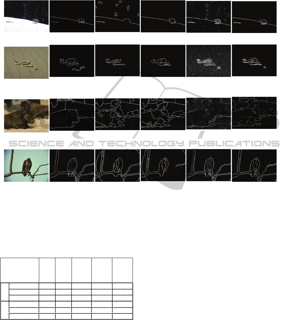
Figure 4 shows some results, where (a) shows

the input image, (b) the human benchmark and the

segmentation result of (c) corresponds to JSEG, (d)

MM-Frac, (e) morphological gradient edge detection

and (f) result of KSS process, already binarized in

the best threshold computed by the BSDS. Each

result has its computed F-measure metric.

In a qualitatively comparison, the original JSEG

algorithm tends to over-segment images, splitting

objects into several smaller regions. The MM-Frac

approach, by its turn, significantly decreases over-

segmentation. For an example, the trees in the

background in the first image are not segmented as

in the JSEG result. Moreover, the results present

more accurate boundaries when compared to the

human benchmark. In the second line, the boundary

encompasses the entire body of the snake and not

fragments.

In the fifth column, the results of edge detection

are presented. The results are very noisy and this is

mainly due to the fact that edge detection techniques

rely entirely on the local information available in the

image. The edge-map responds to all contrast

variations over the texture regions, like in the sand

area on the second line of Figure 4. At the same

time, the method of edge detection is responsible for

highlighting details such as the stick in the left in the

snow area in the first line of Figure 4 and the insect

near to the snake in the second image of Figure 4.

The results for the KSS method are presented in

the last column. Details detected using edge

detection method are kept, but the noise was

attenuated and disappears after the binarization

computed by BSDS. Now, the boundaries are more

accurate and are closer to the human perception.

Deng and Manjunath (2001) pointed out that the

major problem they observed in JSEG result is

caused by the varying shades due to the illumination.

For instance, the color of a sky can vary in a very

smooth transition as in the image BSDS image

42049, the last line of Figure 4. Visually, there is no

clear boundary. However, the JSEG result presents a

circle region in the image. The human perception

does not perceive this smooth varying of color as a

different region. The result after KSS does not

present this false boundary. The smooth is not

perceived by the edge detection, and then the

boundary is erased by the KSS method.

Quantitatively speaking, the metrics recall,

precision and F-measure of each method computed

by the BSDS are tabbed in the superior part of Table

MM-Frac approach improves the recall metric

without decreasing precision, thus raising the F-

measure score a little bit. Edge detection looses in

terms of precision, because of the noisy pixels.

VISAPP 2011 - International Conference on Computer Vision Theory and Applications

184

Input Image

Human

Benchmark

JSEG MM-Frac Edge Detection KSS

167062 F-measure = 0.95

F-measure = 0.62

F-measure=0.88

F-measure=0.92

F-measure=0.94

196073

F-measure = 0.85

F-measure=0.55

F-measure=0.74 F-measure=0.70

F-measure=0.79

41033

F-measure = 0.88

F-measure=0.56 F-measure=0.62

F-measure=0.60

F-measure = 0.66

42049

(a)

F-measure = 0.96

(b)

F-measure = 0.75

(c)

F-measure = 0.58

(d)

F-measure = 0.93

(e)

F-measure = 0.91

(f)

Figura 4: (a) Input image (b) Human benchmark (c) JSEG result (d) MM-Frac result (e) Edge Detection result (f) KSS

result in the best threshold.

After KSS method, the F-measure increases to 0.61,

this is the closest value, comparing to the human

perception.

Table 1: Metrics of each method computed by BSDS.

Human

JSEG

MM-Frac

Edge

Detection

After

KSS

Recall 0.70 0.61 0.63 0.65 0.69

Precision 0.89 0.56 0.56 0.49 0.54

F-measure 0.79 0.58 0.59 0.56 0.61

Recall 0.70 0.61 0.63 0.69 0.73

Precision 0.89 0.57 0.57 0.55 0.57

F-measure 0.78 0.58 0.59 0.59 0.63

BSDS computes the maximum F-measure value

across the precision-recall curve, for which each

point corresponds to an image in the test dataset.

Differently, bottom part of Table 1 shows the

average value of the same three metrics, for the one

hundred images available in the test dataset. From

such average values, the advantage of the proposed

two-level strategy becomes much clearer.

4 CONCLUSIONS

This work proposes a new two-level approach to

boundary detection for natural color images. In the

first level we embedded a MM in the classical JSEG

algorithm. The integration, called MM-Frac, is

controlled by the slope of the image power

spectrum. One conclusion is that the MM improves

the sensitivity to boundary regions, thus providing

segmentation results that match the human

perception better than the segmentation results

associated with the original JSEG algorithm.

In the second-level, the post-processing

integration, the main goal is to integrate the region-

growing result from MM-Frac and edge information.

Our strategy, called KSS, is to put together the two

maps, eliminating the false boundaries in region-

TWO-LEVEL STRATEGY FOR IMAGE BOUNDARY DETECTION

185

map, based on edge information, and eliminating the

noisy edges in the edge-map, based on region

information. The KSS algorithm works well and

solves the problem of false boundaries pointed out in

other works. Furthermore, all strong edges of both

input maps are held, improving the boundary

detection. Unfortunately, the KSS results present

broken edges, not keeping the contour closed.

The conclusion is that the two-level approach

proposed here improves the boundary detection

results, generating segmented images that match the

human perception better than the results associated

to the individual methods used in the architecture.

ACKNOWLEDGEMENTS

The authors would like to thank CAPES (Brazil) for

financial support.

REFERENCES

Chaudhuri, B. B.; Sarkar, N., 1995. Texture segmentation

using fractal dimension, IEEE Trans. Pattern Anal.

Mach. Intell., 17 (1), 72–77.

Côco, K. F., Salles, E. O. T., Sarcinelli-Filho, M., 2009.

Topographic independent component analysis based

on fractal and morphology applied to texture

segmentation, Lecture Notes in Computer Science,

5441, 491-498.

Deng, Y., Manjunath, B. S., 2001. Unsupervised

segmentation of color-texture regions in images and

video, IEEE Trans. Pattern Anal. Mach. Intell., 23 (8).

Komati, K. S., Salles, E. O. T., Sarcinelli-Filho, M., 2010.

Unsupervised color image segmentation based on local

fractal dimension, In Proc. 17th International

Conference on Systems, Signals and Image Processing

(IWSSIP 2010), 1, 243-246.

Komati, K. S., Salles, E. O. T., Sarcinelli-Filho, M., in

press. A Strategy for Image Boundary Detection

Combining Region and Edge Maps, Computing in

Science and Engineering, IEEE computer Society

Digital Library. doi: 10.1109/MCSE.2010.148.

Martin, D., Fowlkes, C., Tal, D., Malik, J., 2001. A

database of human segmented natural images and its

application to evaluating segmentation algorithms and

measuring ecological statistics, In Proc. 8th IEEE Int´l

Conf. Computer Vision, 2, 416–423.

Martin, D. R., Fowlkes, C. C., Malik, J., 2004. Learning to

detect natural image boundaries using local brightness,

color, and texture cues, IEEE Trans. Pattern Anal.

Mach. Intell., 26(5), 530–549, 2004.

Muñoz, X., Freixenet, J., Cufí, X., Martí, J., 2003.

Strategies for image segmentation combining region

and boundary information, IEEE Pattern Recognition

Letters, 24(1-3), 375–392.

Pentland, A. P., 1984 Fractal-based description of natural

scenes. IEEE Trans. on Pattern Analysis and Machine

Intelligence, 6.

Rotem, O., Greenspan, H., Goldberger, J., 2007.

Combining Region and Edge Cues for Image

Segmentation in a Probabilistic Gaussian Mixture

Framework. In Proc 2007 IEEE Conference on

Computer Vision and Pattern Recognition, 1-8.

Torralba, A., Oliva, A., 2003. Statistics of natural image

categories, Institute of Physics Publishing:

Computation in Neural Systems, 14, 391-412.

VISAPP 2011 - International Conference on Computer Vision Theory and Applications

186