TEXTURE CLASSIFICATION USING SPARSE K-SVD TEXTON

ICTIONARIES

Muhammad Rushdi and Jeffrey Ho

Computer and Information Science and Engineering, University of Florida, Gainesville, U.S.A.

Keywords:

Texture classiﬁcation, Texton, Sparse representation, Image dictionary.

Abstract:

This paper addresses the problem of texture classiﬁcation under unknown viewpoint and illumination vari-

ations. We propose an approach that combines sparse K-SVD and texton-based representations. Starting

from an analytic or data-driven base dictionary, a sparse dictionary is iteratively estimated from the texture

data using the doubly-sparse K-SVD algorithm. Then, for each texture image, K-SVD representations of pixel

neighbourhoods are computed and used to assign the pixels to textons. Hence, the texture image is represented

by the histogram of its texton map. Finally, a test image is classiﬁed by ﬁnding the closest texton histogram

using the chi-squared distance. Initial experiments on the CUReT database show high classiﬁcation rates that

compare well with Varma-Zisserman MRF results.

1 INTRODUCTION

The problem of classifying texture images under un-

known viewpoint and illumination variations is a

challenging task. The difﬁculty of the problem stems

from several facts. Firstly, images of the same mate-

rial with large variations of the pose, illumination, or

scale may appear so different even for a human ob-

server. Secondly, techniques that are accurate, adapt-

able and fast need to be developed to predict cor-

rectly the classes of new texture images in a reason-

able amount of time.

Indeed, a lot of work has been done in the area

of texture classiﬁcation (Davies, 2008), (Varma and

Zisserman, 2009), (Liu et al., 2009), (Zhao and

Pietikainen, 2006), (Leung and Malik, 2001), (Cula

and Dana, 2001). Leung and Peterson (Leung and

Peterson, 1992) used moment-invariant and log-polar

features to classify texture. Kang (Kang and Na-

gahashi, 2005) developed a framework for scale-

invariant texture analysis using multi-scale local au-

tocorrelation features. Dana et al created the CUReT

database (Dana et al., 1999) which contains texture

images for 61 categories where each category is rep-

resented by 205 images of different viewing and il-

lumination conditions. Varma and Zisserman devel-

oped several texture classiﬁers based on ﬁlter banks

(Varma and Zisserman, 2002) and image patch ex-

emplars (Varma and Zisserman, 2009). Hayman et

al (Hayman and Eklundh, 2004) created the KTH-

TIPS texture database (Fritz and Eklundh, 2004) that

samples texture at multiple illumination, poses and

scales. As well, they devised an SVM-based approach

to classify texture.

Our contribution in this paper is to introduce a

novel texture classiﬁcation algorithm that combines

the sparse K-SVD representation with texton-based

systems. We give some background materials, ex-

plain our method, then report the results of our ex-

periments.

2 BACKGROUND

2.1 Sparse K-SVD Algorithm

Elad et al (Rubinstein et al., 2010) deﬁne a model

for sparse signal representation, the sparse dictionary

model, where the signal dictionary D is decomposed

into a pre-speciﬁed base dictionary Φ and a sparse

dictionary A

D = ΦA.

(1)

In this model, let the sparse signal representation γ

has a maximum of t non-zero elements. As well, each

column of A is normalized and has a maximum of

p non-zero elements. To train a sparse dictionary, we

need to approximatelysolve the optimization problem

187

Rushdi M. and Ho J..

TEXTURE CLASSIFICATION USING SPARSE K-SVD TEXTON DICTIONARIES.

DOI: 10.5220/0003376101870193

In Proceedings of the International Conference on Computer Vision Theory and Applications (VISAPP-2011), pages 187-193

ISBN: 978-989-8425-47-8

 2011 SCITEPRESS (Science and Technology Publications, Lda.)

minimize

A,Γ

kX− ΦAΓk

subject to



∀i kΓ

≤ t

∀ j ka

≤ p, kΦa

= 1.

(2)

In this expression, the columns of Γ are the sparse K-

SVD representations of the corresponding columns of

the dataset X, and the function k.k

counts the non-

zero entries of a vector. Solving this problem is car-

ried out by alternating sparse-coding and dictionary

update steps for a ﬁxed number of iterations. The

sparse-coding step can be efﬁciently implemented

using orthogonal matching pursuits (OMP) (Davis

et al., 1997). The sparse dictionary model strikes a

balance between complexity (via the choice of the

base dictionary Φ) and adaptability (via the training

of the sparse dictionary A). As well, training the

sparse dictionary is less time-consuming, less prone

to noise and instability, and more computationally ef-

ﬁcient than that of explicit dictionaries. This what

makes this model appealing for pattern recognition

tasks.

2.2 Varma-Zisserman Texture Classiﬁer

Varma and Zisserman introduced a texture classiﬁer

based on image patch exemplars (Varma and Zisser-

man, 2009). This approach can be summarized as fol-

lows. Firstly, all images are made zero-mean and unit-

variance. Secondly, image patches of N × N window

size are taken and reordered in N

-dimensional fea-

ture space. Thirdly, image patches are contrast nor-

malized using Weber’s law

F(x) ← F(x)[log(1+ L(x)/0.03)]/L(x)

(3)

where L(x) = kF(x)k

is the magnitude of the patch

vector at that pixel x. Fourthly, all of the image

patches from the selected training images in a tex-

ture class are aggregated and clustered using the k-

means algorithm. The set of the cluster centres from

all classes form the texton dictionary. Fifthly, training

(and testing) images are modelled by the histogram of

texton frequencies. Finally, novel image classiﬁcation

is achieved by nearest-neighbour matching using the

statistic. This classiﬁer is known as the joint clas-

siﬁer. One important variant of the joint classiﬁer is

the MRF classiﬁer which explicitly models the joint

distribution of the central pixels and their neighbours.

Refer to (Varma and Zisserman, 2009) for further de-

tails.

3 SPARSE K-SVD

TEXTON-BASED TEXTURE

CLASSIFIER

Our goal is to build a texture classiﬁcation system us-

ing a combination of sparse-coding and texton tech-

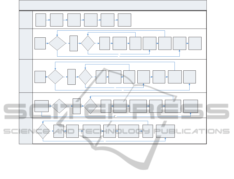
niques. A cross-functional ﬂowchart of the system is

shown in Figure 1. The ﬂowchart consists of the fol-

lowing stages:

3.1 Parameter Setup

Several parameters need to be speciﬁed for the sparse

K-SVD algorithm. These parameters include the

block (or window) size, the base dictionary size and

model, the sparse dictionary size, the sparsity of the

sparse dictionary with respect to the base dictionary,

the sparsity of the image patch K-SVD representa-

tion with respect to the sparse dictionary, the sparse-

coding criteria (sparsity-based or error-based), the

number of iterations for estimating the sparse dictio-

nary. Refer to (Rubinstein et al., 2010) for further

information on these parameters. As well, for classi-

ﬁcation with textons, we need to specify the window

size (which must be the same as the K-SVD block

size), the size of the texton dictionary, and the num-

ber bins for the MRF variant of the Varma-Zisserman

classiﬁer.

3.2 Building the Base Dictionary

In this work, we focus on separable base dictionaries

since theyhavecompact representation, sub-quadratic

implementation, and memory-efﬁcient computation.

A separable dictionary is the Kronecker product of

several one-dimensional dictionaries. We consider

here two types of these dictionaries: analytic and

data-driven dictionaries. Analytic dictionaries are de-

ﬁned using standard signal bases like the DCT, over-

complete DCT, and wavelet dictionaries. Data-driven

dictionaries are generated from the given image data

using some clustering schemes such as k-means clus-

tering, or median-based clustering. Speciﬁcally, for

each category c,1 ≤ c ≤ C where C is the number

of texture classes, we sample image blocks from all

of training images, convert the blocks into columns,

apply Weber’s law to contrast-normalize the columns

(Varma and Zisserman, 2009), and then we apply the

clustering scheme to ﬁnd the class-speciﬁc base dic-

tionary Φ

. Then, we concatenate the class-speciﬁc

base dictionaries to get the overall base dictionary Φ

Φ = [Φ

|Φ

|...|Φ

(4)

VISAPP 2011 - International Conference on Computer Vision Theory and Applications

188

KSVD-Based Texture Classification

Compare Test and

Training Maps

Create Training

Texton Maps

Create Sparse Dictionary Create Base Dictionary

Set KSVD

Parameters

Set

block

size

Set sparse

dictionary

size

Set base

dictionary

size and

model

Set signal

and

dictionary

sparsities

Set sparse

coding

criteria

Set

memory

usage

level

Initialize

Base

dictionary

categories?

Images?

Get next

image

Normalize

image

Set image

blocks as

columns

Get class-

specific

base

dictionary

Get

class

Update

global

base

dictionary

Factor

global

base

dictionary

Save

Global

base

dictionary

Y Y

Get next

image

Set image

blocks as

columns

Update

global

sparse

dictionary

Images?

Initialize

sparse

dictionary

Normalize

image

Get class-

specific

sparse

dictionary

categories?

Get

class

Get class-

specific

texton

dictionary

Get global

KSVD

texton

dictionary

Y Y

Initialize

training

histograms

Get

class

Find KSVD

representation

Normalize

image

Get next

image

Compute

texton

histogram

Images?

Update

class-specific

histogram set

Save global

histogram

training set

Find KSVD

representation

Compute

texton

histogram

Normalize

image

Get next

image

Find the Chi-

Squared distance

to all training

histograms

Images?

Find the

output

class

Compute

confusion matrix

and total

success rate

categories?

Figure 1: Cross-functional block diagram of the Sparse K-SVD Texton-Based Texture Classiﬁer.

In Section 4, we give more details on creating data-

driven dictionaries and subsequently converting them

into separable forms.

3.3 Building the Sparse Dictionary

Once the separable base dictionary is generated (an-

alytically or from data), we move on to estimating a

sparse dictionary of the texture data with some spar-

sity level p. To guarantee that each texture category

is fairly represented in the sparse dictionary, we esti-

mate a sub-dictionary for each category then join the

sub-dictionaries to from the whole sparse dictionary.

Speciﬁcally, for each category c,1 ≤ c ≤ C whereC is

the number of texture classes, we estimate a solution

of the optimization problem

minimize

,Γ

− ΦA

subject to



∀i kΓ

≤ t

∀ j ka

≤ p, kΦa

= 1.

(5)

then we concatenate the class-speciﬁc dictionaries to

get the overall sparse dictionary A

A = [A

|...|A

(6)

3.4 Building the Texton Dictionary

We generate a texton dictionary of the texture data as

follows. Firstly, for each category c,1 ≤ c ≤ C where

C is the number of texture classes, we apply a cluster-

ing algorithm to ﬁnd the centroids of the texture class.

Secondly, we join all of the class-speciﬁc centroids to

form the texton dictionary X

textons

. Thirdly, we apply

sparse-coding techniques (e.g. orthogonal matching

pursuit) to X

textons

to ﬁnd the corresponding K-SVD

representation Γ

textons

= argmin

textons

− ΦAΓk

subject to ∀ikΓ

≤ t.

(7)

Note that the size of the texton dictionary should be

small to get reasonable processing times for test tex-

ture images.

3.5 Computing the Image Texton

Histograms

For each training or test image, we follow a texton-

based approach to ﬁnd the texton histogram of the im-

age. Firstly, we convert each pixel and its neighbour-

hood into a column. Secondly, we sparse-code the

TEXTURE CLASSIFICATION USING SPARSE K-SVD TEXTON DICTIONARIES

189

columnized neighbourhood x

by solving the mini-

mization problem

= argmin

− ΦAγk

subject to kγk

≤ t.

(8)

Thirdly, we assign each pixel to the closest texton in

the texton dictionary. Indeed, the Euclidean distance

is measured between the K-SVD representation γ

the pixel neighbourhood and each element of the K-

SVD representation of the texton dictionary Γ

textons

This step produces the texton map of the image. Fi-

nally, we compute the frequency histogram of the tex-

ton map with respect to the textons. This produces a

vector with a length equal to the size of texton dic-

tionary. Alternatively, a texture image may be rep-

resented by an MRF model (Varma and Zisserman,

2009).

3.6 Classifying Test Images

Given a test texture image, its texton frequency his-

togram is computed as described above. Then the dis-

tances between this histogram and all of the training

image texton histograms are measured using the χ

statistic where

(x,y) =

∑

− y

)

+ y

(9)

4 CONSTRUCTION OF

DATA-DRIVEN SEPARABLE

IMAGE DICTIONARIES

As we mentioned in Section 3.2, a separable im-

age dictionary may be found from data by applying

clustering methods then approximating the resulting

dictionary by a Kronecker product of 1D dictionary

components. One advantage of this base dictionary

construction approach is that the resulting dictionary

closely represents the population of texture classes.

This is in contrast to an analytic dictionary (e.g. DCT

or wavelets) that might be too generic to represent

the texture data set. A second advantage can be real-

ized if we use clustering schemes that represent each

cluster by one of its members (e.g. k-Medoids algo-

rithms). In this case, representations of image patches

and sparse dictionary atoms will have a direct physi-

cal interpretation in terms of actual points in the tex-

ture data. Now, we give further implementation de-

tails of this base dictionary construction approach.

4.1 Clustering Approaches for Image

Dictionaries

There are numerous clustering approaches in the

literature (Duda et al., 2001), (Theodoridis and

Koutroumbas, 2009). We will focus here on two of

them: k-means, and k-medoids algorithms. The k-

means algorithm is a popular and well-known algo-

rithm. It aims to move the cluster representatives

, j = 1,...,M (where M is the number of clusters)

into regions that are dense in points of the dataset

X by minimizing the sum of squared Euclidean dis-

tances between vectors x

,i = 1,...,N (where N is the

number of data points) and cluster means θ

. The k-

means algorithm is computationally simple and works

well for large datasets. However, the k-means algo-

rithm is sensitive to outliers and noise. As well, k-

means is not suitable for data with nominal or ﬁnite

discrete-valued domains.

Another family of clustering algorithms is the k-

medoids algorithms. In the k-medoids methods, each

cluster is represented by a vector selected among the

elements of X, which is usually referred to as the

medoid. These methods overcome the problems of

k-means. First, k-medoids methods are applicable to

data sets from both continuous and discrete domains.

Second, k-medoids methods are less sensitive to out-

liers and noise. However, these methods are more

computationally demanding than k-means. In particu-

lar, a basic version of the k-medoidsmethods, the Par-

titioning Around Medoids (PAM) algorithm, is pro-

hibitively slow and memory-intensive for clustering

of large datasets. To avoid this problem, another vari-

ant of the k-medoids methods, the Clustering LARge

Applications (CLARA) algorithm, exploits the idea of

randomized sampling in the following way. CLARA

draws randomly a sample X

′

of size N

′

from the en-

tire data set X and then determines the set Θ

′

that best

represents X

′

using the PAM algorithm. The rationale

behind CLARA is that if the sample X

′

is statistically

representative of X , then the set Θ

′

will be a satis-

factory approximation of the set Θ of the medoids

that would result if the PAM algorithm was run on

the whole dataset X (Theodoridis and Koutroumbas,

2009).

4.2 Approximation of Separable

Dictionaries with Kronecker

Products

Once a data-driven dictionary is constructed by clus-

tering, we need to convert it into a separable form.

This can be achieved by approximating the dictionary

VISAPP 2011 - International Conference on Computer Vision Theory and Applications

190

as the Kronecker product of 1D dictionaries. This

problem can be stated as follows. Let the base dictio-

nary Φ ∈ R

m×n

be an m-by-n matrix with m = m

and n = n

. We need to solve the minimization

problem

minimize

,Φ

kΦ− Φ

⊗ Φ

subject to



∈ R

×n

∈ R

×n

(10)

Loan and Pitsianis (Loan and Pitsianis, 1993) approx-

imately solve this problem as follows. Firstly, it is

shown that this problem is equivalent to

minimize

,Φ

kR (Φ) − vec(Φ

)vec(Φ

)

subject to



∈ R

×n

∈ R

×n

(11)

where R (Φ) is the column rearrangement of Φ (rela-

tive to the blocking parameters m

, and n

) and

vec(Φ

),vec(Φ

) are columnized arrangements of Φ

and Φ

, respectively.

Secondly, if

Φ = R (Φ) has singular value decompo-

sition

ΦV = Σ = diag(σ

)

(12)

where σ

is the largest singular value, and U(:,1),V(:

,1) are the corresponding singular vectors, then the

matrices Φ

∈ R

×n

,Φ

∈ R

×n

deﬁned by

vec(Φ

) = σ

U(:, 1)

vec(Φ

) = V(:,1)

(13)

minimize kΦ − Φ

⊗ Φ

(Golub and Loan, 1989).

5 EXPERIMENTS AND RESULTS

5.1 Experimental Texture Data

We performed our texture classiﬁcation experiments

on the Columbia-Utrecht Reﬂectance and Transmis-

sion (CUReT) texture image database (Dana et al.,

1999). The database contains images of 61 texture

materials. Each material has 205 images taken un-

der different viewing and illumination conditions. In

(Varma and Zisserman, 2009), Varma and Zisserman

picked a subset of 92 images for each class. For this

subset, a sufﬁciently large portion of the texture is vis-

ible across all materials. A central 200× 200 region

was cropped from each of the selected images and the

remaining background was discarded. The selected

regions where converted to gray scale, then normal-

ized to zero-mean and unit-variance. This cropped

CUReT database (Varma and Zisserman, 2009) has a

total of 61× 92 images. We use this cropped CUReT

database in our experiments. For each class, 46 im-

ages are randomly chosen for training and the remain-

ing 46 are used for testing.

5.2 Implementation Details

As we mentioned in Section 3, several parame-

ters needs to be experimentally set in our system.

Based on experiments, we found reasonable operat-

ing ranges for some parameters as follows. The size

of the base dictionary was set between 80 and 400 de-

pending on the sparse dictionary size. Much larger

base dictionary adversely affected the performance.

The sparsity of the sparse dictionary was set to values

between 7 and 10 depending on the sizes of the base

and sparse dictionaries. Sparsity of the K-SVD repre-

sentation vectors was set between 11 and 15 depend-

ing on the size of the sparse dictionary. The number

of training iterations was ﬁxed at 30. A block size

of 8 × 8 was chosen as it gave the best classiﬁcation

rate. A sparsity-based sparse-coding (SC) was found

to give better results than error-based criteria. For the

texton dictionary, 10 textons per class were computed

giving a total of 61 × 10 = 610 textons. Increasing

the texton beyond this increased the complexity with

negligible improvement in performance. We tested

both the joint and the MRF classiﬁer variants of the

Varma-Zisserman classiﬁers. We eventually chose to

focus on the MRF variant as it consistently exhibited

better performance. The number of MRF bins was set

to 90. For the CLARA clustering method, 10 random

samples were drawn from the data to ﬁnd the cluster

medoids. The size of the drawn sample was set to

′

= 40+ 2M where M is the number of base dictio-

nary clusters (set between 4 and 7 per class).

5.3 Base Dictionary Model Selection

For the K-SVD base dictionary model, we tried stan-

dard DCT dictionaries , and data-driven dictionaries

generated by the CLARA clustering method (as de-

scribed in Section 4). As we can see from Table

1, using a DCT base dictionary gives better results

than the data-driven CLARA base dictionary. Our in-

terpretation is that the DCT base dictionary covers a

wider range of image structures than the clustering-

based dictionary that we used. This can be veriﬁed

by visualizing both dictionaries and their respective

sparse dictionaries. Figures 2, 3 show sample atoms

of the base dictionaries and the corresponding sparse

dictionaries for best DCT and CLARA results of Ta-

ble 1. It is clearly noticeable that the DCT has more

image structures than the CLARA dictionary. This

TEXTURE CLASSIFICATION USING SPARSE K-SVD TEXTON DICTIONARIES

191

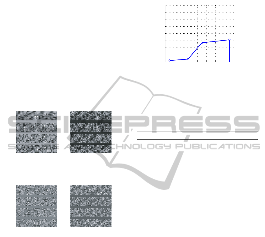
Table 1: Comparison of the classiﬁcation performance of

the sparse K-SVD texture classiﬁer for different choices of

base dictionary construction method (DCT versus CLARA)

and different values of the per-class sparse dictionary size.

Given the 61 CUReT classes, the total sparse dictionary

sizes are 2× 61 = 122 and 9× 61 = 549, respectively.

Per-class A size / Φ Method DCT CLARA

2 92.19% 91.80%

9 94.62% 92.48%

in turn is reﬂected on the richness of the associated

sparse dictionaries. We still think that data-driven

base dictionaries constitute a good choice if the un-

derlying data is well-chosen to cover the texture data

variability. We plan to examine this in future work.

Base Dictionary Sparse Dictionary

Figure 2: Sample atoms from the DCT base dictionary and

its corresponding sparse dictionary for the best DCT-based

result of Table 1.

Base Dictionary Sparse Dictionary

Figure 3: Sample atoms from the CLARA base dictio-

nary and its corresponding sparse dictionary for the best

CLARA-based result of Table 1.

5.4 Spare Dictionary Sizing

The sparse dictionary A size is particularly impor-

tant since it widely affects the running time during

dictionary learning, training, and testing. As well,

this dictionary size clearly affects the classiﬁcation

rate (as shown in Figure 4). The best classiﬁca-

tion rate of 95.12% is achieved at a dictionary size

of 15 × 61 = 915. Increasing the sparse dictionary

size beyond that would give better results but at a high

computational cost.

5.5 Comparison to other Work

Table 2 compares our method with the Varma-

Zisserman patch-based classiﬁers. Despite that our

2 4 6 8 10 12 14 16

100

Perclass Sparse Dictionary Size

Classification Rate

Figure 4: Effect of the per-class sparse dictionary size on

the overall classiﬁcation rate. The best classiﬁcation rate of

95.12% is achieved at a dictionary size of 15× 61 = 915.

Table 2: Comparison of the classiﬁcation performance of

our method with the Varma-Zisserman patch-based classi-

ﬁers. Despite that our method is slightly sub-optimal it has

other advantages such as design ﬂexibility, immunity to out-

liers, sparse representation, and physical interpretation.

Ours VZ Joint VZ Neighbour VZ MRF

95.12% 96.16% 96.08 % 97.47%

method is slightly sub-optimal, it has some potential

advantages that are mainly inherited from the sparse

K-SVD structure. First, complexity can be well mod-

elled through the choice of an analytic or a data-

driven base dictionary. Second, adaptability to data

is achieved through training of the sparse dictionary

component. Third, the sparse representation reduces

the space and time computational complexities. Fi-

nally, sparse signals and dictionary atoms can be as-

cribed direct interpretations in terms of few base dic-

tionary elements. We explore these ideas further in

future work.

6 CONCLUSIONS AND FUTURE

WORK

We introduced a novel texture classiﬁcation algorithm

that combines the sparse K-SVD representation with

texton-based systems. Our system carries the beneﬁts

of the sparse K-SVD algorithm into the texture clas-

siﬁcation problem: sparse representation, adaptabil-

ity to data, and efﬁcient computation. In particular,

we explored the idea of using data-driven base dictio-

naries instead of standard analytical ones to represent

more specialized texture data. Results of the simula-

tions and experiments show that our system closely

matches the state-of-the-art algorithms. In the future,

we will focus on performing better design of the base

and sparse dictionaries. As well, we pursue methods

for optimal parameter selection.

VISAPP 2011 - International Conference on Computer Vision Theory and Applications

192

REFERENCES

Cula, O. and Dana, K. (2001). Compact representation of

bidirectional texture functions. volume 1, pages I–

1041 – I–1047 vol.1.

Dana, K., Van-Ginneken, B., Nayar, S., and Koenderink,

J. (1999). Reﬂectance and Texture of Real World

Surfaces. ACM Transactions on Graphics (TOG),

18(1):1–34.

Davies, E. (2008). Handbook of Texture Analysis, chap-

ter Introduction to Texture Analysis. Imperial College

Press.

Davis, G., Mallat, S., and Avellaneda, M. (1997). Greedy

adaptive approximation. J. Constr. Approx., 13:57–98.

Duda, R., Hart, P., and Stork, D. (2001). Pattern Classiﬁca-

tion. Wiley.

Fritz, M., H. L. C. B. and Eklundh, J.-O. (2004). The

kth-tips database. available at www.nada.kth.se/cvap/

databases/kth-tips.

Golub, G. and Loan, C. V. (1989). Matrix Computations.

John Hopkins Press.

Hayman, L., C. B. and Eklundh, J.-O. (2004). On the sig-

niﬁcance of real-world conditions for material classi-

ﬁcation. In 8th European Conference on Computer

Vision, pages 253–266.

Kang, Y., M. K. and Nagahashi, H. (2005). Scale Space

and PDE Methods in Computer Vision, volume 3459,

chapter Scale Invariant Texture Analysis Using Multi-

scale Local Autocorrelation Features, pages 363–373.

Springer.

Leung, M. and Peterson, A. (1992). Scale and rotation

invariant texture classiﬁcation. In The Twenty-Sixth

Asilomar Conference on Signals, Systems and Com-

puters, volume 1, pages 461–465.

Leung, T. and Malik, J. (2001). Representing and recog-

nizing the visual appearance of materials using three-

dimensional textons. International Journal of Com-

puter Vision, 43.

Liu, G., Lin, Z., and Yu, Y. (2009). Radon representation-

based feature descriptor for texture classiﬁcation. Im-

age Processing, IEEE Transactions on, 18(5):921 –

928.

Loan, C. V. and Pitsianis, N. (1993). Approximation with

kronecker products. In Linear Algebra for Large Scale

and Real Time Applications, pages 293–314. Kluwer

Publications.

Rubinstein, R., Zibulevsky, M., and Elad, M. (2010). Dou-

ble sparsity: Learning sparse dictionaries for sparse

signal approximation. Signal Processing, IEEE Trans-

actions on, 58(3):1553 –1564.

Theodoridis, S. and Koutroumbas, K. (2009). Pattern

Recognition, 4th Edition. Academic Press.

Varma, M. and Zisserman, A. (2002). Classifying images of

materials: Achieving viewpoint and illumination inde-

pendence.

Varma, M. and Zisserman, A. (2009). A statistical ap-

proach to material classiﬁcation using image patch ex-

emplars. IEEE Transactions on Pattern Analysis and

Machine Intelligence, 31(11):2032–2047.

Zhao, G. and Pietikainen, M. (2006). Local binary pattern

descriptors for dynamic texture recognition. volume 2,

pages 211 –214.

TEXTURE CLASSIFICATION USING SPARSE K-SVD TEXTON DICTIONARIES

193