
ACTION RECOGNITION BASED ON MULTI-LEVEL
REPRESENTATION OF 3D SHAPE
Binu M. Nair and Vijayan K. Asari
Department of Electrical and Computer Engineering, University of Dayton, Dayton, Ohio, U.S.A.
Keywords:
Spacetime shape, Radon transform, Distance transform, Shape descriptor.
Abstract:
A novel algorithm has been proposed for recognizing human actions using a combination of shape descrip-
tors. Every human action is considered as a 3D space time shape and the shape descriptors based on the 3D
Euclidean distance transform and the Radon transform are used for its representation. The Euclidean distance
transform gives a suitable internal representation where the interior values correspond to the action performed.
By taking the gradient of this distance transform, the space time shape is divided into different number of
levels with each level representating a coarser version of the original space time shape. Then, at each level and
at each frame, the Radon transform is applied from where action features are extracted. The action features
are the R-Transform feature set which gives the posture variations of the human body with respect to time and
the R-Translation vector set which gives the translatory variation. The combination of these action features is
used in a nearest neighbour classifier for action recognition.
1 INTRODUCTION
Human action recognition has been a widely re-
searched area in computer vision as it holds a lot of
applications relating to security and surveillance. One
such application is the human action detection and
recognition algorithm implemented in systems using
CCTV cameras where the system is used for detecting
suspicious human behavior and alerting the authori-
ties accordingly (C. J .Cohen et al., 2008). Another
area is in object recognition where, by evaluating the
human interaction with the object and recognizing the
human action, the particular object is recognized (M.
Mitani et al., 2006). Thus arises the need for faster
and robust algorithms for human action recognition.
Action recognition involves the extraction of
suitable distinguishable features representing certain
variations in the human body caused due to the action.
One approach involves the use of 2D or 3D shape de-
scriptors to represent a space time shape which is a
concatenation of human silhouettes across time. An-
other approach involves the computation of certain lo-
calised motion fields and trajectories of specific points
from a space time shape. The various invariant prop-
erties extracted from these motion fields and trajecto-
ries are then considered as action features. In the algo-
rithm proposed in this paper, a combination of shape
descriptors are used for the representation of the space
time shape and the extraction of action features. This
algorithm is closely related to the action recognition
framework based on Poisson’s shape descriptor (M.
Blank et al., 2005) and the shape descriptor based on
the Radon transform (Y. Wang et al., 2007).
In the next section, a review of the algorithms that
have been proposed over the last few years for action
recognition, is explained briefly. The algorithms de-
scribed are mainly based on the motion fields and the
shape descriptors. In the third section, the proposed
algorithm for action recognition is explained in detail
with illustrations. Results are provided in the fourth
section where the recognition rates are compared with
those of other algorithms. The variation of the accu-
racies with respect to certain parameters of the algo-
rithm are also given. Finally, the paper concludes the
algorithm by mentioning the pros and cons and dis-
cusses the improvements and the future work.
2 PREVIOUS WORK
In this section, we shall go through some of the works
which are based on motion fields, shape descriptors
and trajectories of tracked body parts.
378
M. Nair B. and K. Asari V..
ACTION RECOGNITION BASED ON MULTI-LEVEL REPRESENTATION OF 3D SHAPE.
DOI: 10.5220/0003376303780386
In Proceedings of the International Conference on Computer Vision Theory and Applications (VISAPP-2011), pages 378-386
ISBN: 978-989-8425-47-8
Copyright
c
2011 SCITEPRESS (Science and Technology Publications, Lda.)
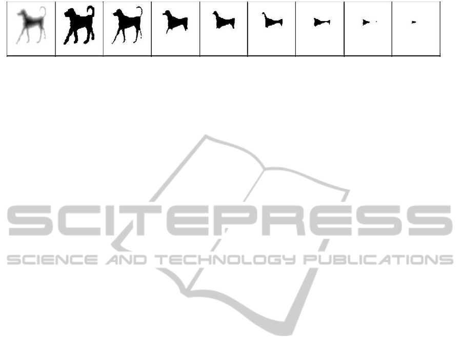
Figure 1: Segmentation of Dog silhouette given in (S.Tabbone et al., 2006).
2 PREVIOUS WORK
In this section, we shall go through some of the works
which are based on motion fields, shape descriptors
and trajectories of tracked body parts.
2.1 Algorithms Based on Motion
Capture Fields or Trajectories
Earlier works in action recognition makes use of
temporal templates such as motion history images
(J.W.Davis and A.F.Bobick, 1997), the timed mo-
tion history images (G.R.Bradski and J.W.Davis,
2000) and the hierarchical motion history images
(J.W.Davis, 2003) where these templates provides the
motion characteristics such as the motion history im-
age and motion energy image at every spatial location
of a frame in an image sequence. Some of the features
extracted are the optical flow vectors from the MHI
gradient, the radial histogram and local and global
orientation computed at each pixel (G.R.Bradski and
J.W.Davis, 2000). The speed of motion of a body
movement was incorporated by computing the MHI
from scaled versions of the images and extracting the
motion fields from each level (J.W.Davis, 2003).
Motion descriptors based purely on the optical
flow measurements computed from each pixel of
the video frame are used to describe an action of
an individual at a far off distance from the camera
(A.A.Efros et al., 2003). These optical flow mea-
surements are calculated from a figure-centric spatio-
temporal volume using the Lucas-Kanade algorithm.
The time variation of the optical flow vector computed
is considered as an action feature which are compared
by a correlation based similarity measure.
Algorithms proposed in (J.C.Niebles et al., 2006;
P.Scovanner et al., 2007) consider action features as
codewords in a codebook where these features are ex-
tracted from interest regions in a space time shape.
In (J.C.Niebles et al., 2006), the interest regions are
the local maxima regions of a response function de-
fined by a combination of a Gaussian and a Gabor
filter computed at every frame and the extracted fea-
tures are the gradient and the optical flow from these
regions while in (P.Scovanner et al., 2007), the inter-
est regions are obtained by random sampling of the
pixels at different locations, time and scale and the
3D SIFT descriptors extracted from these regions are
taken as the action features.
Some of the works proposed a particular model
which includes tracking or segmenting of various
parts of the human body. In (S.Ali et al., 2007), hu-
man actions have been modelled as a non-linear dy-
namical system where the state variables are defined
by the reference joints in the human body silhouette
and their functions are defined by their trajectories.
Here, action features are derived by analysing the tra-
jectories as a time series data and extracting the in-
variant properties. Many methods are available for
studying the time series data but the one used here
applies the theory of chaotic systems to analyze the
non-linear nature (J.Zhang et al., 1998).
The concept of mid-level features known as space
time shapelets is introduced in (D.Batra et al., 2008)
where these shapelets are local volumetric objects or
local 3D shapes extracted from a space time shape.
Thus, an action is represented by a combination of
such shapelets as these represent the motion charac-
teristics on a more localised level. Extracting all the
possible such volumes from each space time shape
of the database and clustering these sub-volumes pro-
vides the cluster centers which are then considered as
space time shapelets.
2.2 Algorithms Based on Shape
Descriptors
Shape descriptors (D.Zhang and G.Lu, 2003; Q.Chen
et al., 2004; A.Khotanzad and Y.H.Hong, 1990;
M.K.Hu, 2008) can be used to extract the variation of
the silhouettes across the video frames. Better vari-
ations can be extracted using shape descriptors such
as the one based on Poisson’s equation (L.Gorelick
et al., 2004) and the one based on the Radon transform
(S.Tabbone et al., 2006). This is because they not only
give the boundary representation of a silhouette of a
3D shape but also give an internal representation. A
brief discussion on these algorithms will be provided
as these form the basis for the algorithm proposed in
this paper.
In (M.Blank et al., 2005), the concept of a space
time shape is introduced where a space time shape
Figure 1: Segmentation of Dog silhouette given in (S. Tabbone et al., 2006).
2.1 Algorithms based on Motion
Capture Fields or Trajectories
Earlier works in action recognition makes use of tem-
poral templates such as motion history images (J.
W. Davis and A. F. Bobick, 1997), the timed mo-
tion history images (G. R. Bradski and J.W.Davis,
2000) and the hierarchical motion history images (J.
W. Davis, 2003) where these templates provides the
motion characteristics such as the motion history im-
age and motion energy image at every spatial loca-
tion of a frame in an image sequence. Some of the
features extracted are the optical flow vectors from
the MHI gradient, the radial histogram and local and
global orientation computed at each pixel (G. R. Brad-
ski and J.W.Davis, 2000). The speed of motion of a
body movement was incorporated by computing the
MHI from scaled versions of the images and extract-
ing the motion fields from each level (J. W. Davis,
2003).
Motion descriptors based purely on the optical
flow measurements computed from each pixel of the
video frame are used to describe an action of an in-
dividual at a far off distance from the camera (A. A.
Efros et al., 2003). These optical flow measurements
are calculated from a figure-centric spatio-temporal
volume using the Lucas-Kanade algorithm. The time
variation of the optical flow vector computed is con-
sidered as an action feature which are compared by a
correlation based similarity measure.
Algorithms proposed in (J. C. Niebles et al., 2006;
P. Scovanner et al., 2007) consider action features as
codewords in a codebook where these features are ex-
tracted from interest regions in a space time shape.
In (J. C. Niebles et al., 2006), the interest regions are
the local maxima regions of a response function de-
fined by a combination of a Gaussian and a Gabor
filter computed at every frame and the extracted fea-
tures are the gradient and the optical flow from these
regions while in (P. Scovanner et al., 2007), the inter-
est regions are obtained by random sampling of the
pixels at different locations, time and scale and the
3D SIFT descriptors extracted from these regions are
taken as the action features.
Some of the works proposed a particular model
which includes tracking or segmenting of various
parts of the human body. In (S. Ali et al., 2007), hu-
man actions have been modelled as a non-linear dy-
namical system where the state variables are defined
by the reference joints in the human body silhouette
and their functions are defined by their trajectories.
Here, action features are derived by analysing the tra-
jectories as a time series data and extracting the in-
variant properties. Many methods are available for
studying the time series data but the one used here
applies the theory of chaotic systems to analyze the
non-linear nature (J. Zhang et al., 1998).
The concept of mid-level features known as space
time shapelets is introduced in (D. Batra et al., 2008)
where these shapelets are local volumetric objects or
local 3D shapes extracted from a space time shape.
Thus, an action is represented by a combination of
such shapelets as these represent the motion charac-
teristics on a more localised level. Extracting all the
possible such volumes from each space time shape
of the database and clustering these sub-volumes pro-
vides the cluster centers which are then considered as
space time shapelets.
2.2 Algorithms based on Shape
Descriptors
Shape descriptors (D. Zhang and G. Lu, 2003; Q.
Chen et al., 2004; A. Khotanzad and Y. H. Hong,
1990; M. K. Hu, 2008) can be used to extract the vari-
ation of the silhouettes across the video frames. Bet-
ter variations can be extracted using shape descrip-
tors such as the one based on Poisson’s equation (L.
Gorelick et al., 2004) and the one based on the Radon
transform (S. Tabbone et al., 2006). This is because
they not only give the boundary representation of a
silhouette of a 3D shape but also give an internal rep-
resentation. A brief discussion on these algorithms
will be provided as these form the basis for the algo-
rithm proposed in this paper.
In (M. Blank et al., 2005), the concept of a space
time shape is introduced where a space time shape
is formed by the concatenation of silhouettes in the
video frames and considering actions as 3D shapes.
The shape descriptors based on the Poisson’s equa-
tion in 3D used to represent the space time shape and
various properties such as local space-time saliency,
shape structure, action dynamics and local orientation
ACTION RECOGNITION BASED ON MULTI-LEVEL REPRESENTATION OF 3D SHAPE
379

are extracted. A shape descriptor based on the Radon
transform (R. N. Bracewell, 1995) known as the R-
Transform is defined in (Y. Wang et al., 2007). This
transform is used to represent the low-level features
in a binary silhouette in a single frame and these are
used in the training of hidden Markov models to rec-
ognize the action.
A combination of shape flow and motion flow
features have been used as action features in
(A.Mohiuddin and S.W.Lee, 2008) where the shape
flow features are a combination of different moment
based shape descriptors and the motion flow feature
is the optical flow. The shape descriptors used are
the Hu’s invariant moments (M. K. Hu, 2008) and
Zernike moments (A. Khotanzad and Y. H. Hong,
1990). In (X. Sun et al., 2009), instead of using op-
tical flow feature vectors to represent the local fea-
tures, both 2D and 3D SIFT descriptors are used while
the global features extracted are the Zernike moments
from the motion energy images. The 2D SIFT de-
scriptor emphasizes the 2D silhouette shape and the
3D SIFT descriptor emphasizes the motion.
3 MULTI-LEVEL SHAPE
REPRESENTATION
We shall first review the multi-level representation of
a 2D shape using the R-Transform which is proposed
in (S. Tabbone et al., 2006). First, the distance trans-
form (G. Borgefors, 1984; D. W. Paglieroni, 1992; A.
Rosenfeld and J. Pfaltz, 1966) based on the Euclidean
distance is computed for that shape. The computation
involves the approximation of the Euclidean distance
transform and this approximation is the (3,4) Chamfer
distance transform. Using the values obtained from
the transform, the 2D shape is segmented into dif-
ferent levels using a predefined threshold. The levels
correspond to the coarseness of the shape and this is
illustrated in Figure 1. As shown, the silhoutte of a
dog has been segmented into 8 different levels. Now,
at each of these levels, the R-transform is computed
which can be defined as
R
f
(α) =
Z
+∞
−∞
T
2
(s,α)ds (1)
where T (s,α) is the radon transform of the 2D bi-
nary image. As proved in (S. Tabbone et al., 2006),
the R-Transform is translation invariant and is made
scale invariant by normalizing it with its area. Since
it is not rotation invariant, the scaled magnitude of
the discrete Fourier transform is computed. There-
fore, the multi-level representation of 2D shape is the
set of magnitudes of the discrete Fourier transform of
the R-Transform at each level of the shape.
4 PROPOSED ALGORITHM
The proposed algorithm is an application of the multi-
level shape representation to a space time shape which
provides the necessary features of action classifica-
tion. The 3D Euclidean distance transform (P. F.
Felzenszwalb and D. P. Huttenlocher, 2004) gives the
internal representation where its gradient is used to di-
vide the space time shape into different levels. Then,
at each level, the R-Transform and the R-Translation
features are extracted and these are considered as suit-
able action features. The various steps involved in the
algorithm are explained in detail in this section.
is formed by the concatenation of silhouettes in the
video frames and considering actions as 3D shapes.
The shape descriptors based on the Poisson’s equa-
tion in 3D used to represent the space time shape and
various properties such as local space-time saliency,
shape structure, action dynamics and local orienta-
tion are extracted. A shape descriptor based on the
Radon transform (R.N.Bracewell, 1995) known as the
R-Transform is defined in (Y.Wang et al., 2007). This
transform is used to represent the low-level features
in a binary silhouette in a single frame and these are
used in the training of hidden Markov models to rec-
ognize the action.
A combination of shape flow and motion flow
features have been used as action features in
(A.Mohiuddin and S.W.Lee, 2008) where the shape
flow features are a combination of different moment
based shape descriptors and the motion flow feature
is the optical flow. The shape descriptors used are the
Hu’s invariant moments (M.K.Hu, 2008) and Zernike
moments (A.Khotanzad and Y.H.Hong, 1990). In
(X.Sun et al., 2009), instead of using optical flow fea-
ture vectors to represent the local features, both 2D
and 3D SIFT descriptors are used while the global
features extracted are the Zernike moments from the
motion energy images. The 2D SIFT descriptor em-
phasizes the 2D silhouette shape and the 3D SIFT de-
scriptor emphasizes the motion.
3 MULTI-LEVEL SHAPE
REPRESENTATION
We shall first review the multi-level representation
of a 2D shape using the R-Transform which is pro-
posed in (S.Tabbone et al., 2006). First, the dis-
tance transform (G.Borgefors, 1984; D.W.Paglieroni,
1992; A.Rosenfeld and J.Pfaltz, 1966) based on the
Euclidean distance is computed for that shape. The
computation involves the approximation of the Eu-
clidean distance transform and this approximation is
the (3,4) Chamfer distance transform. Using the val-
ues obtained from the transform, the 2D shape is seg-
mented into different levels using a predefined thresh-
old. The levels correspond to the coarseness of the
shape and this is illustrated in Figure 1. As shown, the
silhoutte of a dog has been segmented into 8 different
levels. Now, at each of these levels, the R-transform
is computed which can be defined as
R
f
(α) =
Z
+∞
−∞
T
2
(s,α)ds (1)
where T (s,α) is the radon transform of the 2D bi-
nary image. As proved in (S.Tabbone et al., 2006),
the R-Transform is translation invariant and is made
scale invariant by normalizing it with its area. Since
it is not rotation invariant, the scaled magnitude of
the discrete Fourier transform is computed. There-
fore, the multi-level representation of 2D shape is the
set of magnitudes of the discrete Fourier transform of
the R-Transform at each level of the shape.
4 PROPOSED ALGORITHM
The proposed algorithm is an application of the multi-
level shape representation to a space time shape
which provides the necessary features of action clas-
sification. The 3D Euclidean distance transform
(P.F.Felzenszwalb and D.P.Huttenlocher, 2004) gives
the internal representation where its gradient is used
to divide the space time shape into different lev-
els. Then, at each level, the R-Transform and the R-
Translation features are extracted and these are con-
sidered as suitable action features. The various steps
involved in the algorithm are explained in detail in
this section.
Figure 2: Extraction of a silhouette from a video frame.
Figure 3: Space time shapes of jumping jack and walk ac-
tions.
4.1 Silhouette Extraction and
Formation of Space-time shapes.
First, the silhouettes are extracted from each frame of
the video sequence by comparing it with its median
background and then, thresholding, dilating and erod-
ing to form the binary silhouette image shown in Fig-
ure 2. Once the silhouettes are extracted, a predefined
number are concatenated to form the 3D space time
Figure 2: Extraction of a silhouette from a video frame.
is formed by the concatenation of silhouettes in the
video frames and considering actions as 3D shapes.
The shape descriptors based on the Poisson’s equa-
tion in 3D used to represent the space time shape and
various properties such as local space-time saliency,
shape structure, action dynamics and local orienta-
tion are extracted. A shape descriptor based on the
Radon transform (R.N.Bracewell, 1995) known as the
R-Transform is defined in (Y.Wang et al., 2007). This
transform is used to represent the low-level features
in a binary silhouette in a single frame and these are
used in the training of hidden Markov models to rec-
ognize the action.
A combination of shape flow and motion flow
features have been used as action features in
(A.Mohiuddin and S.W.Lee, 2008) where the shape
flow features are a combination of different moment
based shape descriptors and the motion flow feature
is the optical flow. The shape descriptors used are the
Hu’s invariant moments (M.K.Hu, 2008) and Zernike
moments (A.Khotanzad and Y.H.Hong, 1990). In
(X.Sun et al., 2009), instead of using optical flow fea-
ture vectors to represent the local features, both 2D
and 3D SIFT descriptors are used while the global
features extracted are the Zernike moments from the
motion energy images. The 2D SIFT descriptor em-
phasizes the 2D silhouette shape and the 3D SIFT de-
scriptor emphasizes the motion.
3 MULTI-LEVEL SHAPE
REPRESENTATION
We shall first review the multi-level representation
of a 2D shape using the R-Transform which is pro-
posed in (S.Tabbone et al., 2006). First, the dis-
tance transform (G.Borgefors, 1984; D.W.Paglieroni,
1992; A.Rosenfeld and J.Pfaltz, 1966) based on the
Euclidean distance is computed for that shape. The
computation involves the approximation of the Eu-
clidean distance transform and this approximation is
the (3,4) Chamfer distance transform. Using the val-
ues obtained from the transform, the 2D shape is seg-
mented into different levels using a predefined thresh-
old. The levels correspond to the coarseness of the
shape and this is illustrated in Figure 1. As shown, the
silhoutte of a dog has been segmented into 8 different
levels. Now, at each of these levels, the R-transform
is computed which can be defined as
R
f
(α) =
Z
+∞
−∞
T
2
(s,α)ds (1)
where T (s,α) is the radon transform of the 2D bi-
nary image. As proved in (S.Tabbone et al., 2006),
the R-Transform is translation invariant and is made
scale invariant by normalizing it with its area. Since
it is not rotation invariant, the scaled magnitude of
the discrete Fourier transform is computed. There-
fore, the multi-level representation of 2D shape is the
set of magnitudes of the discrete Fourier transform of
the R-Transform at each level of the shape.
4 PROPOSED ALGORITHM
The proposed algorithm is an application of the multi-
level shape representation to a space time shape
which provides the necessary features of action clas-
sification. The 3D Euclidean distance transform
(P.F.Felzenszwalb and D.P.Huttenlocher, 2004) gives
the internal representation where its gradient is used
to divide the space time shape into different lev-
els. Then, at each level, the R-Transform and the R-
Translation features are extracted and these are con-
sidered as suitable action features. The various steps
involved in the algorithm are explained in detail in
this section.
Figure 2: Extraction of a silhouette from a video frame.
Figure 3: Space time shapes of jumping jack and walk ac-
tions.
4.1 Silhouette Extraction and
Formation of Space-time shapes.
First, the silhouettes are extracted from each frame of
the video sequence by comparing it with its median
background and then, thresholding, dilating and erod-
ing to form the binary silhouette image shown in Fig-
ure 2. Once the silhouettes are extracted, a predefined
number are concatenated to form the 3D space time
Figure 3: Space time shapes of jumping jack and walk ac-
tions.
4.1 Silhouette Extraction and
Formation of Space-time Shapes
First, the silhouettes are extracted from each frame of
the video sequence by comparing it with its median
background and then, thresholding, dilating and erod-
ing to form the binary silhouette image shown in Fig-
ure 2. Once the silhouettes are extracted, a predefined
number are concatenated to form the 3D space time
shapes with axes x,y and t. The space time shapes are
shown in Figure 3.
VISAPP 2011 - International Conference on Computer Vision Theory and Applications
380
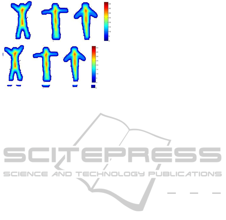
Figure 4: Sample Frames of the distance transformed space
time shape formed from 10 silhouttes.
Figure 5: Sample frames of the gradient of the distance
transformed shape.
shapes with axes x, y and t. The space time shapes are
shown in Figure 3.
4.2 Computation of Euclidean Distance
Transform
To segment the space time shape, the 3D distance
transform (P.F.Felzenszwalb and D.P.Huttenlocher,
2004) based on the Euclidean distance is computed.
This transformation assigns to a interior voxel a value
which is proportional to the Euclidean distance be-
tween this voxel and the nearest boundary voxel. The
computation involves the use of a 3-pass algorithm
where each pass is associated with a raster scan of the
entire space time shape in a particular dimension us-
ing a 1D mask.
The minimum distance calculation is done by
finding the local minima of the lower envelope of the
set of parabolas where each parabola is defined on the
basis of the Euclidean distance between two points
(P.F.Felzenszwalb and D.P.Huttenlocher, 2004). The
intermediate distance transform vales computed in the
first pass is based directly on the Euclidean distance.
In the next two passes, the distance transform values
are computed from the set of parabolas defined on the
boundary voxels in the respective dimension. This
type of distance transform is given by
D
f
(p) = min
qε B
((p − q)
2
+ f (q)) (2)
where p is a non-boundary point, q is a boundary
point, B is the boundary and f (q) is the value of the
distance measure between points p and q. It is seen
that for every qεB, the distance transform is bounded
by the parabola rooted at (q, f (q)). In short, the dis-
tance transform value at point p is the minima of the
lower envelope of the parabolas formed from every
boundary point q. The distance transformation of the
space time shape is shown in Figure 4. It is seen
that the area covered by the torso part of the body
has higher values than the area covered by the limbs.
By varying the aspect ratio, the different axes x,y and
t will have different emphasis on the computed dis-
tance transform.
4.3 Segmentation of the 3D Space-time
Shape
Human actions are distinguished from the variation
of the silhouette and these variations are more along
the limbs than in the torso. So, a better representation
of the space time shape is required which emphasizes
fast moving parts so that the features extracted gives
the necessary variation to represent the action. Thus, a
normalized gradient of the distance transform is used
and, as shown in Figure 5, the fast moving parts such
as the limbs have higher values compared to the torso
region. The gradient of the space time shape φ(x,y,t)
(M.Blank et al., 2005) is defined as
φ(x,y,t) = U (x,y,t) +K
1
·
∂
2
U
∂x
2
+K
2
·
∂
2
U
∂y
2
+K
3
·
∂
2
U
∂t
2
(3)
Figure 6: 8-Level segmentation of sample frames of the
space time shape of the “Jumping-Jack” action.
where U(x,y,t) is the distance transformed space time
shape, K
i
is the weight added to the derivative taken
along the i
th
axis. The weights associated with the
Figure 4: Sample Frames of the distance transformed space
time shape formed from 10 silhouttes.
Figure 4: Sample Frames of the distance transformed space
time shape formed from 10 silhouttes.
Figure 5: Sample frames of the gradient of the distance
transformed shape.
shapes with axes x,y and t. The space time shapes are
shown in Figure 3.
4.2 Computation of Euclidean Distance
Transform
To segment the space time shape, the 3D distance
transform (P.F.Felzenszwalb and D.P.Huttenlocher,
2004) based on the Euclidean distance is computed.
This transformation assigns to a interior voxel a value
which is proportional to the Euclidean distance be-
tween this voxel and the nearest boundary voxel. The
computation involves the use of a 3-pass algorithm
where each pass is associated with a raster scan of the
entire space time shape in a particular dimension us-
ing a 1D mask.
The minimum distance calculation is done by
finding the local minima of the lower envelope of the
set of parabolas where each parabola is defined on the
basis of the Euclidean distance between two points
(P.F.Felzenszwalb and D.P.Huttenlocher, 2004). The
intermediate distance transform vales computed in the
first pass is based directly on the Euclidean distance.
In the next two passes, the distance transform values
are computed from the set of parabolas defined on the
boundary voxels in the respective dimension. This
type of distance transform is given by
D
f
(p) = min
qε B
((p − q)
2
+ f (q)) (2)
where p is a non-boundary point, q is a boundary
point, B is the boundary and f (q) is the value of the
distance measure between points p and q. It is seen
that for every qεB, the distance transform is bounded
by the parabola rooted at (q, f (q)). In short, the dis-
tance transform value at point p is the minima of the
lower envelope of the parabolas formed from every
boundary point q. The distance transformation of the
space time shape is shown in Figure 4. It is seen
that the area covered by the torso part of the body
has higher values than the area covered by the limbs.
By varying the aspect ratio, the different axes x,y and
t will have different emphasis on the computed dis-
tance transform.
4.3 Segmentation of the 3D Space-time
Shape
Human actions are distinguished from the variation
of the silhouette and these variations are more along
the limbs than in the torso. So, a better representation
of the space time shape is required which emphasizes
fast moving parts so that the features extracted gives
the necessary variation to represent the action. Thus, a
normalized gradient of the distance transform is used
and, as shown in Figure 5, the fast moving parts such
as the limbs have higher values compared to the torso
region. The gradient of the space time shape φ(x,y,t)
(M.Blank et al., 2005) is defined as
φ(x,y,t) = U(x, y,t)+K
1
·
∂
2
U
∂x
2
+K
2
·
∂
2
U
∂y
2
+K
3
·
∂
2
U
∂t
2
(3)
Figure 6: 8-Level segmentation of sample frames of the
space time shape of the “Jumping-Jack” action.
where U(x,y,t) is the distance transformed space time
shape, K
i
is the weight added to the derivative taken
along the i
th
axis. The weights associated with the
Figure 5: Sample frames of the gradient of the distance
transformed shape.
4.2 Computation of Euclidean Distance
Transform
To segment the space time shape, the 3D distance
transform (P. F. Felzenszwalb and D. P. Huttenlocher,
2004) based on the Euclidean distance is computed.
This transformation assigns to a interior voxel a value
which is proportional to the Euclidean distance be-
tween this voxel and the nearest boundary voxel. The
computation involves the use of a 3-pass algorithm
where each pass is associated with a raster scan of the
entire space time shape in a particular dimension us-
ing a 1D mask.
The minimum distance calculation is done by
finding the local minima of the lower envelope of the
set of parabolas where each parabola is defined on the
basis of the Euclidean distance between two points (P.
F. Felzenszwalb and D. P. Huttenlocher, 2004). The
intermediate distance transform vales computed in the
first pass is based directly on the Euclidean distance.
In the next two passes, the distance transform values
are computed from the set of parabolas defined on the
boundary voxels in the respective dimension. This
type of distance transform is given by
D
f
(p) = min
qεB
((p − q)
2
+ f (q)) (2)
where p is a non-boundary point, q is a boundary
point, B is the boundary and f (q) is the value of the
distance measure between points p and q. It is seen
that for every q εB, the distance transform is bounded
by the parabola rooted at (q, f (q)). In short, the dis-
tance transform value at point p is the minima of the
lower envelope of the parabolas formed from every
boundary point q. The distance transformation of the
space time shape is shown in Figure 4. It is seen
that the area covered by the torso part of the body
has higher values than the area covered by the limbs.
By varying the aspect ratio, the different axes x,y and
t will have different emphasis on the computed dis-
tance transform.
4.3 Segmentation of the 3D Space-time
Shape
Human actions are distinguished from the variation
of the silhouette and these variations are more along
the limbs than in the torso. So, a better representation
of the space time shape is required which emphasizes
fast moving parts so that the features extracted gives
the necessary variation to represent the action. Thus, a
normalized gradient of the distance transform is used
and, as shown in Figure 5, the fast moving parts such
as the limbs have higher values compared to the torso
region. The gradient of the space time shape φ(x,y,t)
(M. Blank et al., 2005) is defined as
φ(x,y,t) = U(x,y,t) + K
1
·
∂
2
U
∂x
2
+K
2
·
∂
2
U
∂y
2
+K
3
·
∂
2
U
∂t
2
(3)
Figure 4: Sample Frames of the distance transformed space
time shape formed from 10 silhouttes.
Figure 5: Sample frames of the gradient of the distance
transformed shape.
shapes with axes x,y and t. The space time shapes are
shown in Figure 3.
4.2 Computation of Euclidean Distance
Transform
To segment the space time shape, the 3D distance
transform (P.F.Felzenszwalb and D.P.Huttenlocher,
2004) based on the Euclidean distance is computed.
This transformation assigns to a interior voxel a value
which is proportional to the Euclidean distance be-
tween this voxel and the nearest boundary voxel. The
computation involves the use of a 3-pass algorithm
where each pass is associated with a raster scan of the
entire space time shape in a particular dimension us-
ing a 1D mask.
The minimum distance calculation is done by
finding the local minima of the lower envelope of the
set of parabolas where each parabola is defined on the
basis of the Euclidean distance between two points
(P.F.Felzenszwalb and D.P.Huttenlocher, 2004). The
intermediate distance transform vales computed in the
first pass is based directly on the Euclidean distance.
In the next two passes, the distance transform values
are computed from the set of parabolas defined on the
boundary voxels in the respective dimension. This
type of distance transform is given by
D
f
(p) = min
qε B
((p − q)
2
+ f (q)) (2)
where p is a non-boundary point, q is a boundary
point, B is the boundary and f (q) is the value of the
distance measure between points p and q. It is seen
that for every qεB, the distance transform is bounded
by the parabola rooted at (q, f (q)). In short, the dis-
tance transform value at point p is the minima of the
lower envelope of the parabolas formed from every
boundary point q. The distance transformation of the
space time shape is shown in Figure 4. It is seen
that the area covered by the torso part of the body
has higher values than the area covered by the limbs.
By varying the aspect ratio, the different axes x,y and
t will have different emphasis on the computed dis-
tance transform.
4.3 Segmentation of the 3D Space-time
Shape
Human actions are distinguished from the variation
of the silhouette and these variations are more along
the limbs than in the torso. So, a better representation
of the space time shape is required which emphasizes
fast moving parts so that the features extracted gives
the necessary variation to represent the action. Thus, a
normalized gradient of the distance transform is used
and, as shown in Figure 5, the fast moving parts such
as the limbs have higher values compared to the torso
region. The gradient of the space time shape φ(x, y,t)
(M.Blank et al., 2005) is defined as
φ(x,y,t) = U (x,y,t)+K
1
·
∂
2
U
∂x
2
+K
2
·
∂
2
U
∂y
2
+K
3
·
∂
2
U
∂t
2
(3)
Figure 6: 8-Level segmentation of sample frames of the
space time shape of the “Jumping-Jack” action.
where U(x, y,t) is the distance transformed space time
shape, K
i
is the weight added to the derivative taken
along the i
th
axis. The weights associated with the
Figure 6: 8-Level segmentation of sample frames of the
space time shape of the “Jumping-Jack” action.
where U(x,y,t) is the distance transformed space time
shape, K
i
is the weight added to the derivative taken
along the i
th
axis. The weights associated with the
gradients along each of the axes are usually kept the
same. It is seen that the proper variation occurs where
the time axis has more emphasis. The fast moving
parts in this case being the hands and legs have high
values, the region surrounding the torso which are not
so fast moving have moderate values while the torso
region which moves very slowly with respect to the
limbs have very low values. Moreover this represen-
tation also contains concatenation of silhouettes from
the previous frame onto the current frame due to the
ACTION RECOGNITION BASED ON MULTI-LEVEL REPRESENTATION OF 3D SHAPE
381
gradient and so, the time nature is emphasized in a
single frame of the space time shape. In short, this
representation of the space time shape is tuned more
towards the time variation where this variation is di-
rectly related to the action being performed. The nor-
malized gradient L(x,y,t) is given by
L(x,y,t) =
log(φ(x, y,t))
max
(x,y,t)ε S
(φ(x,y,t))
(4)
gradients along each of the axes are usually kept the
same. It is seen that the proper variation occurs where
the time axis has more emphasis. The fast moving
parts in this case being the hands and legs have high
values, the region surrounding the torso which are not
so fast moving have moderate values while the torso
region which moves very slowly with respect to the
limbs have very low values. Moreover this represen-
tation also contains concatenation of silhouettes from
the previous frame onto the current frame due to the
gradient and so, the time nature is emphasized in a
single frame of the space time shape. In short, this
representation of the space time shape is tuned more
towards the time variation where this variation is di-
rectly related to the action being performed. The nor-
malized gradient L(x,y,t) is given by
L(x,y,t) =
log(φ(x,y,t))
max
(x,y,t)εS
(φ(x,y,t))
(4)
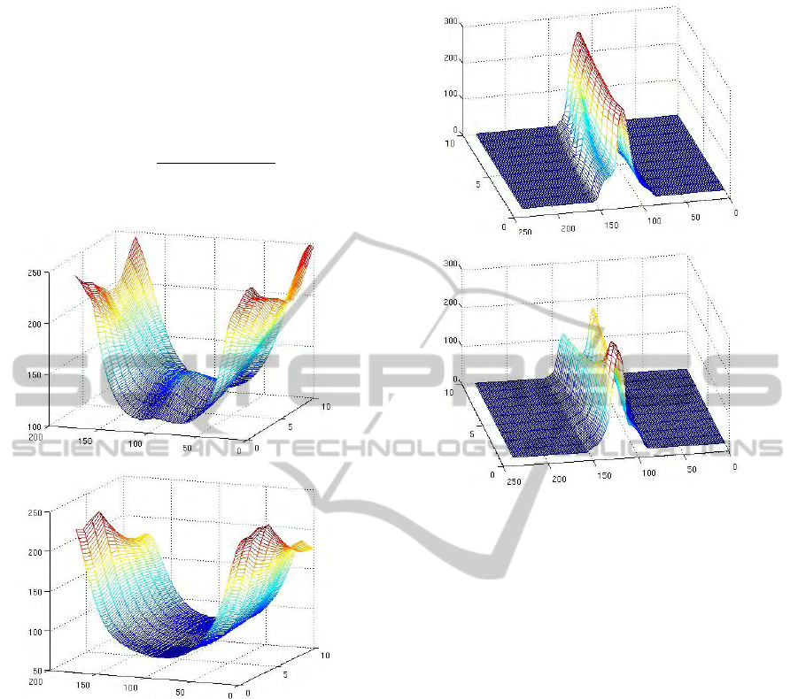
Figure 7: R-Transform Feature Set of the jumping jack and
the walk actions at a finest level.
This normalized gradient is used to segment the
space time shape into multiple levels where at each
level, the features corresponding to the silhouette
variations in a frame are extracted. The standard
deviation of L(x,y,t) is computed to define the in-
Figure 8: R-Translation vector set of the jumping jack and
the walk actions at the coarsest level.
terval between adjacent levels. The interval is de-
fined by s = StdDev/Scale where StdDev is the stan-
dard deviation and Scale is the factor which is usu-
ally taken as 4. The minimum value is taken to be
zero and the threshold for each level is computed as
T h = (p − 1) × s where p refers to the level. For a K
level segmentation, p varies from 1 to K. An illustra-
tion of 8-level segmentation of a space time shape for
different frames are shown in Figure 6. The segmen-
tation is done on each frame using the values of the
normalized gradient and from each level, a particular
set of features are extracted. In the next section, the
type of features extracted from the space time shape
will be discussed.
4.4 Extraction of Features
There are two sets of features which are extracted
from the segmented space time shape. One is the set
of translation invariant R-Transform features obtained
at each level and the other is the R-Translation vectors
which are extracted at the coarsest level of the space
time shape. The R-Transform describes the 2D shape
in a frame at a certain level. The set of R-Transforms
taken across the frames of the space time shape at
Figure 7: R-Transform Feature Set of the jumping jack and
the walk actions at a finest level.
This normalized gradient is used to segment the
space time shape into multiple levels where at each
level, the features corresponding to the silhouette
variations in a frame are extracted. The standard
deviation of L(x, y,t) is computed to define the in-
terval between adjacent levels. The interval is de-
fined by s = StdDev/Scale where StdDev is the stan-
dard deviation and Scale is the factor which is usu-
ally taken as 4. The minimum value is taken to be
zero and the threshold for each level is computed as
T h = (p − 1) × s where p refers to the level. For a K
level segmentation, p varies from 1 to K. An illustra-
tion of 8-level segmentation of a space time shape for
different frames are shown in Figure 6. The segmen-
tation is done on each frame using the values of the
normalized gradient and from each level, a particular
set of features are extracted. In the next section, the
gradients along each of the axes are usually kept the
same. It is seen that the proper variation occurs where
the time axis has more emphasis. The fast moving
parts in this case being the hands and legs have high
values, the region surrounding the torso which are not
so fast moving have moderate values while the torso
region which moves very slowly with respect to the
limbs have very low values. Moreover this represen-
tation also contains concatenation of silhouettes from
the previous frame onto the current frame due to the
gradient and so, the time nature is emphasized in a
single frame of the space time shape. In short, this
representation of the space time shape is tuned more
towards the time variation where this variation is di-
rectly related to the action being performed. The nor-
malized gradient L(x,y,t) is given by
L(x,y,t) =
log(φ(x,y,t))
max
(x,y,t)ε S
(φ(x,y,t))
(4)
Figure 7: R-Transform Feature Set of the jumping jack and
the walk actions at a finest level.
This normalized gradient is used to segment the
space time shape into multiple levels where at each
level, the features corresponding to the silhouette
variations in a frame are extracted. The standard
deviation of L(x,y,t) is computed to define the in-
Figure 8: R-Translation vector set of the jumping jack and
the walk actions at the coarsest level.
terval between adjacent levels. The interval is de-
fined by s = StdDev/Scale where StdDev is the stan-
dard deviation and Scale is the factor which is usu-
ally taken as 4. The minimum value is taken to be
zero and the threshold for each level is computed as
T h = (p − 1) × s where p refers to the level. For a K
level segmentation, p varies from 1 to K. An illustra-
tion of 8-level segmentation of a space time shape for
different frames are shown in Figure 6. The segmen-
tation is done on each frame using the values of the
normalized gradient and from each level, a particular
set of features are extracted. In the next section, the
type of features extracted from the space time shape
will be discussed.
4.4 Extraction of Features
There are two sets of features which are extracted
from the segmented space time shape. One is the set
of translation invariant R-Transform features obtained
at each level and the other is the R-Translation vectors
which are extracted at the coarsest level of the space
time shape. The R-Transform describes the 2D shape
in a frame at a certain level. The set of R-Transforms
taken across the frames of the space time shape at
Figure 8: R-Translation vector set of the jumping jack and
the walk actions at the coarsest level.
type of features extracted from the space time shape
will be discussed.
4.4 Extraction of Features
There are two sets of features which are extracted
from the segmented space time shape. One is the set
of translation invariant R-Transform features obtained
at each level and the other is the R-Translation vectors
which are extracted at the coarsest level of the space
time shape. The R-Transform describes the 2D shape
in a frame at a certain level. The set of R-Transforms
taken across the frames of the space time shape at
each level gives the posture variations corresponding
to a particular action. The R-Translation vector taken
at the coarsest level emphasizes the translatory vari-
ation of the entire silhouette across the frames of the
space time shape while reducing the emphasis on the
posture variations.
4.4.1 R-Transform Feature Set
The R-Transform feature set is the set of elements
where each element is given by
R
k,l
(α) =
Z
∞
−∞
T
2
k,l
(s,α)ds (5)
VISAPP 2011 - International Conference on Computer Vision Theory and Applications
382

where T
k,l
(s,α) is the 2D Radon transform of the
frame k of the space time shape at level l and αε [0, π[
is the angle of inclination of the line on which the sil-
houette in the frame is projected on (S. Tabbone et al.,
2006). For a space time shape containing K frames
and for L number of levels, the R-Transform feature
set is a 3D matrix of size L × M × K where M is the
number of angles on which the projection is taken.
Typically, M is taken as 180. The surface plot for the
R-Transform feature set for a single level is shown in
Figure 7. This gives the posture variations of the sil-
houette across the frames and these differ from action
to action and are independent of the person perform-
ing it. This is due to the fact that the R-Transform is
scale and translation invariant where scale invariance
removes the size variations in the persons performing
the action and the variations captured are only due to
the change of shape. Moreover, being translation in-
variant, the features are also independent of the posi-
tion of the person performing the action.
4.4.2 R-Translation Vector Set
The R-Transform feature set gives the variations of
the silhouette shape across the frames but removes the
variation caused due to the translation of the shape.
Therefore, to distinguish between the actions which
have large translatory motions such as walk and run
actions from those which have very little translatory
motion such as single hand wave action, another set
of features should be extracted which gives the trans-
latory variation while minimizing the time variation
of the shape. This type of feature is known as the
R-Translation vector shown in Figure 8. This fea-
ture vector extracted from a frame k of the space time
shape at the coarsest level, is given by
RT
k
(s) =
Z
π
−π
T
2
k,1
(s,α)dα (6)
where T
k,l
is the 2D Radon transform of the centered
silhouette present at the frame k. The R-translation
vector is obtained by integrating the 2D Radon trans-
form over the variable α. Before the extraction of
the R-Translation vector, the silhouette in every frame
of the space time shape is shifted with respect to the
position of the silhouette in the first frame. The R-
Translation vector is then extracted from the modi-
fied silhouettes and the variation in this vector across
the frames gives the translation of the silhouette. The
set of R-Translation vectors extracted from the space
time shape is a matrix of size K × M where K is the
number of frames and M refers to twice the maxi-
mum distance of the projection line from the centroid
of the silhouette. At every frame k, Figure 8 shows
a Gaussian-like function having a peak at s = M/2
and these Gaussian-like functions do not vary much
across the frames for the jumping jack action but for
the walk action, there is considerable variation. This
shows that the jumping jack action has less transla-
tory motion than the walk action. The small variations
that occur in the R-Translation vectors of the jumping
jack is due to the posture variations but unlike the R-
Transform feature set, the type of variations have less
emphasis in the R-Translation vector.
5 SIMULATION AND RESULTS
The implementation of the algorithm are done using
MATLAB and OPENCV library by calling the nec-
essary functions. The extraction of the silhouettes
is done in C++ using OPENCV (G. Bradski and A.
Kaehler, 2008) while the rest of the algorithm such as
the extraction of R-Translation and R-Transform fea-
tures is done in the MATLAB environment. The train-
ing and the testing is done using the Weizmann action
dataset which consists of 90 low-resolution video se-
quences each having a single person performing a par-
ticular action. Each video sequence is taken at 50 fps
with a frame size of 180 × 144 and the dataset con-
tains 10 different action classes. Space time shapes
are extraced from each of the video sequences by us-
ing a window along the time axis where this win-
dow is of a pre-defined length. The training and
the testing data set thus consists of the space time
shapes extracted from each of the video sequences
in the database. For evaluation of the algorithm, a
variation of the “leave-one-out” procedure (M. Blank
et al., 2005) is used where to test a video sequence,
the space time shapes corresponding to that particu-
lar video sequence is taken as the testing data while
the training data set is the set of space time shapes
extracted from the sequences excluding the test se-
quence. Classification of the test set is done by tak-
ing each test space time shape independently and by
comparing the features extracted from it with those
extracted from the training space time shapes, the in-
dividual test space time shape is classified. The com-
parison is done using the nearest neighbour rule (C.
M. Bishop, 2006) by computing the Euclidean dis-
tance between the features. Once the closest training
space time shape is identified, its class is noted and
the test space time shape is classified under this par-
ticular class. The number of test space time shapes
classified correctly for each class are noted and this is
put up in the form of the confusion matrix. The con-
fusion matrix showing the action recognition rates for
the proposed algorithm are shown in Table 1.
The algorithm is also shown to be somewhat con-
ACTION RECOGNITION BASED ON MULTI-LEVEL REPRESENTATION OF 3D SHAPE
383
sistent with the change in the window size used for ex-
tracting the space time shape and the overlap between
consecutive shapes. Simulations were done with 6
different sets of (length,overlap) of space time shape
- (6,3), (8,4), (10,5), (12,6) ,(14,7) and (16,8) and the
recognition rates for each action achieved with each
of the sets is shown in Figure 10. By performing the
evaluation with different sets of the window size and
overlap, we are inturn evaluating the variation caused
due to the speed of the action. If we assume that for
a space time shape, we have a fixed start frame, then,
by varying the window size, the end frames will dif-
fer. This is the same effect as capturing the same ac-
tion with the same window size but both actions per-
formed at two different speeds. As mentioned before,
there is not much variation in the action accuracies for
each action except the case of the skip where the ac-
curacy drops to a slightly lower value. As long as the
variation in the speed of the action is within a certain
limit, the algorithm is consistent with the recognition
accuracy.
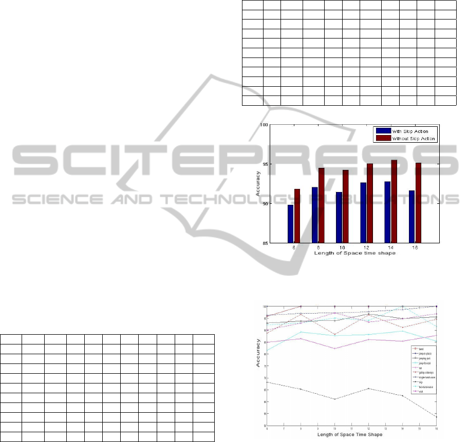
It can be seen that the accuracy for each action
is fairly good enough at around 90 − 95 % with some
actions having an average accuracy of 88 %. But one
particular action, the “skip” action gets an accuracy
of around 60 − 65 %. The impact of this action when
computing the overall accuracy achieved with this al-
gorithm is shown in Figure 9.
Table 1: Confusion Matrix for the Proposed Algorithm. a1
- bend, a2 - jump in place , a3 - jumping jack , a4 - jump
forward , a5 - run , a6 - side , a7 - single-hand wave , a8 -
skip , a9 - double-hand wave , a10 - walk.
a1 a2 a3 a4 a5 a6 a7 a8 a9 a10
a1 100
a2 100
a3 96 3
a4 88 11
a5 86 10 4
a6 96 3
a7 2 97
a8 3 15 65 15
a9 4 1 94
a10 2 1 1 93
It is seen that without including the skip action,
the algorithm achieves a very good overall accu-
racy of around 93 − 95 % accuracy. The inclusion
of the “skip” action reduces the overall accuracy to
90 − 93 %. But even with the “skip” action, the over-
all accuracy is fairly good enough. This reason for
the “skip” action to have a poor accuracy when com-
pared to other actions is due to the fact that some of
the “skip” space time shapes are qualitatively similar
to the “walk” and “run” space time shapes and thus,
they get misclassified under the “walk” and “run” ac-
Table 2: Confusion Matrix for Algorithm using Poisson’s
equation based shape descriptor.a1 - bend, a2 - jump in
place , a3 - jumping jack , a4 - jump forward , a5 - run ,
a6 - side , a7 - single-hand wave , a8 - skip , a9 - double-
hand wave , a10 - walk.
a1 a2 a3 a4 a5 a6 a7 a8 a9 a10
a1 99
a2 100
a3 100
a4 89
a5 98
a6 100
a7 94
a8 97
a9 97
a10 100
comparing the features extracted from it with those
extracted from the training space time shapes, the
individual test space time shape is classified. The
comparison is done using the nearest neighbour rule
(C.M.Bishop, 2006) by computing the Euclidean dis-
tance between the features. Once the closest training
space time shape is identified, its class is noted and
the test space time shape is classified under this par-
ticular class. The number of test space time shapes
classified correctly for each class are noted and this is
put up in the form of the confusion matrix. The con-
fusion matrix showing the action recognition rates for
the proposed algorithm are shown in Table 1.
The algorithm is also shown to be somewhat con-
sistent with the change in the window size used for ex-
tracting the space time shape and the overlap between
consecutive shapes. Simulations were done with 6
different sets of (length,overlap) of space time shape
- (6,3), (8,4), (10,5), (12,6) ,(14,7) and (16,8) and the
recognition rates for each action achieved with each
of the sets is shown in Figure 10. By performing the
evaluation with different sets of the window size and
overlap, we are inturn evaluating the variation caused
due to the speed of the action. If we assume that for
a space time shape, we have a fixed start frame, then,
by varying the window size, the end frames will dif-
fer. This is the same effect as capturing the same ac-
tion with the same window size but both actions per-
formed at two different speeds. As mentioned before,
there is not much variation in the action accuracies for
each action except the case of the skip where the ac-
curacy drops to a slightly lower value. As long as the
variation in the speed of the action is within a certain
limit, the algorithm is consistent with the recognition
accuracy.
It can be seen that the accuracy for each action
is fairly good enough at around 90 − 95 % with some
actions having an average accuracy of 88 %. But one
particular action, the “skip” action gets an accuracy
of around 60 − 65 %. The impact of this action when
computing the overall accuracy achieved with this al-
gorithm is shown in Figure 9.
It is seen that without including the skip action,
the algorithm achieves a very good overall accu-
racy of around 93 − 95 % accuracy. The inclusion
of the “skip” action reduces the overall accuracy to
90 − 93 %. But even with the “skip” action, the over-
all accuracy is fairly good enough. This reason for
the “skip” action to have a poor accuracy when com-
pared to other actions is due to the fact that some of
the “skip” space time shapes are qualitatively similar
to the “walk” and “run” space time shapes and thus,
they get misclassified under the “walk” and “run” ac-
tions. The features extracted capture the more global
Table 1: Confusion Matrix for the Proposed Algorithm. a1
- bend, a2 - jump in place , a3 - jumping jack , a4 - jump
forward , a5 - run , a6 - side , a7 - single-hand wave , a8 -
skip , a9 - double-hand wave , a10 - walk.
a1 a2 a3 a4 a5 a6 a7 a8 a9 a10
a1 100
a2 100
a3 96 3
a4 88 11
a5 86 10 4
a6 96 3
a7 2 97
a8 3 15 65 15
a9 4 1 94
a10 2 1 1 93
Table 2: Confusion Matrix for Algorithm using Poisson’s
equation based shape descriptor.a1 - bend, a2 - jump in
place , a3 - jumping jack , a4 - jump forward , a5 - run ,
a6 - side , a7 - single-hand wave , a8 - skip , a9 - double-
hand wave , a10 - walk.
a1 a2 a3 a4 a5 a6 a7 a8 a9 a10
a1 99
a2 100
a3 100
a4 89
a5 98
a6 100
a7 94
a8 97
a9 97
a10 100
Figure 9: The overall accuracy acheived with and with-
out including the skip action for different space time shape
lengths.
variations of a space time shape and are not able to
fully distinguish between the variations in the “skip”
to that of the “walk” and “run” space time shapes.
One possible way of improving the distinguishability
of these features is to extract another subset of fea-
tures which are more localised and which can provide
more discrimination between the space time shapes.
The confusion matrices for the algorithm which
use the poisson equation’s based shape descriptor is
Figure 9: The overall accuracy acheived with and with-
out including the skip action for different space time shape
lengths.
Figure 10: Accuracy for each action acheived with the dif-
ferent lengths of space time shape. The overlap is half the
length of the space time shape.
Figure 11: Comparison of overall accuracies acheived the
different shape descriptors used in the proposed action
recognition framework without including the “skip” action.
given in Table 2. As seen, the algorithm using the
Poisson’s equation based shape descriptor gives bet-
ter accuracy results for some actions especially the
“skip” action. This is because the features extracted
are localized within the space time shape and thus
are able to fully distinguish between the “skip” and
“walk” shapes. But, the proposed algorithm attains
comparable results with the other actions some ac-
tions attaining better accuracy with the proposed one.
When compared to other shape descriptors, the pro-
posed algorithm uses a combination of shape descrip-
tors which brings out more time variations relating
to the action . This is illustrated in where the shape
descriptor used in the proposed algorithm is com-
pared with other shape descriptors. As shown, the
shape descriptor used in the proposed action recogni-
tion framework has much better overall accuracy than
when acheived with using only the 2D shape descrip-
tors to capture the posture variations.
6 CONCLUSIONS
The algorithm proposed in this paper have used the
concept of a multi-level representation of a 3D shape
for action classification. An action has been consid-
ered as a space time shape or a 3D shape and a multi-
level representation using the gradient of the 3D Eu-
clidean distance transform and the Radon transform
have been used from where the action features have
been extracted. Silhouettes from a video sequence
containing a particular action have been concante-
nated to form the space time shape representing that
action. Action features were extracted from each level
of the representation and these features concatenated
as a single feature was used in a nearest neighbour
classifier for recognition.
The evaluation of the algorithm was performed
by comparing the accuracies attained with different
shape descriptors in the proposed algorithm and the
results obtained showed higher accuracy rates for the
combination of the shape descriptors. Furthur com-
parison has been done with another algorithm pro-
posed in (M.Blank et al., 2005) and the results showed
comparable recognition accuracies for some actions
with some actions having better accuracies with the
proposed one. The accuracies were also computed
for different shape time shape lengths and overlap and
showed that the algorithm was almost consistent with
the variation in the length of the space time shape.
However, the algorithm has not been evaluated for the
variation in the accuracy of a particular action due to
the change in the frame rate as the database used for
evaluation is limited and contains only sequences cap-
tured at a constant frame rate.
Although the average accuracies were high, the
accuracy for one particular action obtained by the pro-
posed algorithm is low as the features extracted from
the space time shape corresponding to this action can-
not be discriminated from those of similar actions.
Future work will involve extraction of weights from
the action features which corresponds to its variation
and then, use a learning based methodolgy to classify
them.
REFERENCES
A.A.Efros, A.C.Berg, G.Mori, and J.Malik (2003). Recog-
nizing action at a distance. In Proceedings of Ninth
IEEE International Conference on Computer Vision.
A.Khotanzad and Y.H.Hong (1990). Invariant image recog-
nition by zernike moments. In IEEE Transactions on
Pattern Analysis and Machine Intelligence.
A.Mohiuddin and S.W.Lee (2008). Human action recogni-
Figure 10: Accuracy for each action acheived with the dif-
ferent lengths of space time shape. The overlap is half the
length of the space time shape.
tions. The features extracted capture the more global
variations of a space time shape and are not able to
fully distinguish between the variations in the “skip”
to that of the “walk” and “run” space time shapes.
One possible way of improving the distinguishability
of these features is to extract another subset of fea-
tures which are more localised and which can provide
more discrimination between the space time shapes.
VISAPP 2011 - International Conference on Computer Vision Theory and Applications
384

Figure 10: Accuracy for each action acheived with the dif-
ferent lengths of space time shape. The overlap is half the
length of the space time shape.
Figure 11: Comparison of overall accuracies acheived the
different shape descriptors used in the proposed action
recognition framework without including the “skip” action.
given in Table 2. As seen, the algorithm using the
Poisson’s equation based shape descriptor gives bet-
ter accuracy results for some actions especially the
“skip” action. This is because the features extracted
are localized within the space time shape and thus
are able to fully distinguish between the “skip” and
“walk” shapes. But, the proposed algorithm attains
comparable results with the other actions some ac-
tions attaining better accuracy with the proposed one.
When compared to other shape descriptors, the pro-
posed algorithm uses a combination of shape descrip-
tors which brings out more time variations relating
to the action . This is illustrated in where the shape
descriptor used in the proposed algorithm is com-
pared with other shape descriptors. As shown, the
shape descriptor used in the proposed action recogni-
tion framework has much better overall accuracy than
when acheived with using only the 2D shape descrip-
tors to capture the posture variations.
6 CONCLUSIONS
The algorithm proposed in this paper have used the
concept of a multi-level representation of a 3D shape
for action classification. An action has been consid-
ered as a space time shape or a 3D shape and a multi-
level representation using the gradient of the 3D Eu-
clidean distance transform and the Radon transform
have been used from where the action features have
been extracted. Silhouettes from a video sequence
containing a particular action have been concante-
nated to form the space time shape representing that
action. Action features were extracted from each level
of the representation and these features concatenated
as a single feature was used in a nearest neighbour
classifier for recognition.
The evaluation of the algorithm was performed
by comparing the accuracies attained with different
shape descriptors in the proposed algorithm and the
results obtained showed higher accuracy rates for the
combination of the shape descriptors. Furthur com-
parison has been done with another algorithm pro-
posed in (M.Blank et al., 2005) and the results showed
comparable recognition accuracies for some actions
with some actions having better accuracies with the
proposed one. The accuracies were also computed
for different shape time shape lengths and overlap and
showed that the algorithm was almost consistent with
the variation in the length of the space time shape.
However, the algorithm has not been evaluated for the
variation in the accuracy of a particular action due to
the change in the frame rate as the database used for
evaluation is limited and contains only sequences cap-
tured at a constant frame rate.
Although the average accuracies were high, the
accuracy for one particular action obtained by the pro-
posed algorithm is low as the features extracted from
the space time shape corresponding to this action can-
not be discriminated from those of similar actions.
Future work will involve extraction of weights from
the action features which corresponds to its variation
and then, use a learning based methodolgy to classify
them.
REFERENCES
A.A.Efros, A.C.Berg, G.Mori, and J.Malik (2003). Recog-
nizing action at a distance. In Proceedings of Ninth
IEEE International Conference on Computer Vision.
A.Khotanzad and Y.H.Hong (1990). Invariant image recog-
nition by zernike moments. In IEEE Transactions on
Pattern Analysis and Machine Intelligence.
A.Mohiuddin and S.W.Lee (2008). Human action recogni-
Figure 11: Comparison of overall accuracies acheived the
different shape descriptors used in the proposed action
recognition framework without including the “skip” action.
The confusion matrices for the algorithm which
use the poisson equation’s based shape descriptor is
given in Table 2. As seen, the algorithm using the
Poisson’s equation based shape descriptor gives bet-
ter accuracy results for some actions especially the
“skip” action. This is because the features extracted
are localized within the space time shape and thus
are able to fully distinguish between the “skip” and
“walk” shapes. But, the proposed algorithm attains
comparable results with the other actions some ac-
tions attaining better accuracy with the proposed one.
When compared to other shape descriptors, the pro-
posed algorithm uses a combination of shape descrip-
tors which brings out more time variations relating
to the action . This is illustrated in where the shape
descriptor used in the proposed algorithm is com-
pared with other shape descriptors. As shown, the
shape descriptor used in the proposed action recogni-
tion framework has much better overall accuracy than
when acheived with using only the 2D shape descrip-
tors to capture the posture variations.
6 CONCLUSIONS
The algorithm proposed in this paper have used the
concept of a multi-level representation of a 3D shape
for action classification. An action has been consid-
ered as a space time shape or a 3D shape and a multi-
level representation using the gradient of the 3D Eu-
clidean distance transform and the Radon transform
have been used from where the action features have
been extracted. Silhouettes from a video sequence
containing a particular action have been concante-
nated to form the space time shape representing that
action. Action features were extracted from each level
of the representation and these features concatenated
as a single feature was used in a nearest neighbour
classifier for recognition.
The evaluation of the algorithm was performed
by comparing the accuracies attained with different
shape descriptors in the proposed algorithm and the
results obtained showed higher accuracy rates for the
combination of the shape descriptors. Furthur com-
parison has been done with another algorithm pro-
posed in (M. Blank et al., 2005) and the results
showed comparable recognition accuracies for some
actions with some actions having better accuracies
with the proposed one. The accuracies were also com-
puted for different shape time shape lengths and over-
lap and showed that the algorithm was almost consis-
tent with the variation in the length of the space time
shape. However, the algorithm has not been evaluated
for the variation in the accuracy of a particular action
due to the change in the frame rate as the database
used for evaluation is limited and contains only se-
quences captured at a constant frame rate.
Although the average accuracies were high, the
accuracy for one particular action obtained by the pro-
posed algorithm is low as the features extracted from
the space time shape corresponding to this action can-
not be discriminated from those of similar actions.
Future work will involve extraction of weights from
the action features which corresponds to its variation
and then, use a learning based methodolgy to classify
them.
REFERENCES
A. A. Efros, A. C. Berg, G. Mori and J.Malik (2003). Rec-
ognizing action at a distance. In Proceedings of Ninth
IEEE International Conference on Computer Vision.
A. Khotanzad and Y. H. Hong (1990). Invariant image
recognition by zernike moments. In IEEE Transac-
tions on Pattern Analysis and Machine Intelligence.
A. Mohiuddin and S. W. Lee (2008). Human action recogni-
tion using shape and clg-motion flow from multi-view
image sequences. In Pattern Recognition.
A. Rosenfeld and J. Pfaltz (1966). Sequential operations in
digital picture processing. In Journal of the Associa-
tion for Computing Machinery.
C. J. Cohen, K. A. Scott, M. J. Huber, S. C. Rowe and F.
Morelli (2008). Behavior recognition architecture for
surveillance applications. In International Workshop
on Applied Imagery and Pattern Recognition - AIPR
2008.
C. M. Bishop (2006). Pattern Recognition and Machine
Learning. Springer.
D. Batra, T. Chen, and R. Sukthankar (2008). Space-time
shapelets for action recognition. In IEEE Workshop
on Motion and Video Computing - WMVC 2008.
ACTION RECOGNITION BASED ON MULTI-LEVEL REPRESENTATION OF 3D SHAPE
385

D. W. Paglieroni (1992). Distance transforms: Properties
and machine vision applications. In Graphical Models
and Image Processing - CVGIP 1992.
D. Zhang and G. Lu (2003). A comparative study on shape
retrieval using fourier descriptors with different shape
signatures. In Journal of Visual Communication and
Image Representation.
G. Borgefors (1984). Distance transformations in arbitrary
dimensions. In Computer Vision, Graphics, and Im-
age Processing.
G. Bradski and A. Kaehler (2008). Learning OpenCV.
O’Reilly Media Inc.
G. R. Bradski and J. W. Davis (2000). Motion segmentation
and pose recognition with motion history gradients.
In Fifth IEEE Workshop on Applications of Computer
Vision.
J. C. Niebles, H. Wang and L. Fei-Fei (2006). Unsu-
pervised learning of human action categories using
spatial-temporal words. In Proceedings of the British
Machine Vision Conference - BMVC 2006.
J. W. Davis (2003). Hierarchical motion history images
for recognizing human motion. In Proceedings of
the IEEE Workshop on Detection and Recognition of
Events in Video.
J. W. Davis and A. F. Bobick (1997). The representation and
recognition of human movement using temporal tem-
plates. In Proceedings of the IEEE Computer Society
Conference on Computer Vision and Pattern Recogni-
tion.
J.Zhang, K. F. Man and J. Y. Ke (1998). Timeseries pre-
diction using lyapunov exponents in embedding phase
space. In International Conference on Systems, Man
and Cybernetics.
L. Gorelick, M. Galun, E. Sharon, R. Basri, and A. Brandt
(2004). Shape representation and classification us-
ing the poisson equation. In Proceedings of the 2004
IEEE Computer Society Conference on Computer Vi-
sion and Pattern Recognition-CVPR 2004.
M. Blank, L. Gorelick, E. Shechtman, M.Irani, and R.Basri
(2005). Actions as space-time shapes. In Tenth IEEE
International Conference on Computer Vision - ICCV
2005.
M. K. Hu (2008). Visual pattern recognition by moment
invariants. In IEEE Workshop on Motion and Video
Computing - WMVC 2008.
M.Mitani, M.Takaya, A.Kojima, and K.Fukunaga (2006).
Environment recognition based on analysis of human
actions for mobile robot. In The 18th International
Conference on Pattern Recognition - ICPR 2006.
P. F. Felzenszwalb and D. P. Huttenlocher (2004). Distance
transforms of sampled functions. In Technical report,
Cornell Computing and Information Science.
P. Scovanner, S. Ali, and M. Shah (2007). A 3-dimensional
sift descriptor and its application to action recognition.
In Proceedings of the 15th ACM International Confer-
ence on Multimedia.
Q. Chen, E. Petriu and X.Yang (2004). A comparative study
of fourier descriptors and hu’s seven moment invari-
ants for image recognition. In Canadian Conference
on Electrical and Computer Engineering.
R. N. Bracewell (1995). Two-Dimensional Imaging. Pren-
tice Hall, Englewood Cliffs, NJ.
S. Ali, A. Basharat and M.Shah (2007). Chaotic invariants
for human action recognition. In IEEE 11th Interna-
tional Conference on Computer Vision - ICCV 2007.
S. Tabbone, L. Wendling and J. P.Salmon (2006). A new
shape descriptor defined on the radon transform. In
Computer Vision and Image Understanding.
X. Sun, M. Chen and A.Hauptmann (2009). Action recog-
nition via local descriptors and holistic features. In
IEEE Computer Society Conference on Computer Vi-
sion and Pattern Recognition Workshops.
Y. Wang, K. Huang and T.Tan (2007). Human activity
recognition based on r-transform. In IEEE Conference
on Computer Vision and Pattern Recognition - CVPR
2007.
VISAPP 2011 - International Conference on Computer Vision Theory and Applications
386
