INTERACTIVE POINT SPREAD FUNCTION SIMULATION

WITH DIFFRACTION AND INTERFERENCE EFFECTS

Tom Cuypers, Tom Mertens, Philippe Bekaert

Expertise Centre for Digital Media, Hasselt University - tUL - IBBT, Hasselt, Belgium

Se Baek Oh

, Ramesh Raskar

MIT Mechanical Engineering, MIT, Cambridge, U.S.A.

MIT MediaLab, MIT, Cambridge, U.S.A.

Keywords:

PSF, Wigner distribution function, Diffraction, Interference, Grating, Monte Carlo.

Abstract:

Interactive simulation of point spread functions is an invaluable tool for evaluating optical designs. We present

an interactive method for simulating the point spread function for designs that require diffraction and interfer-

ence effects. These effects occure when the design contains apertures whose size approaches the wavelength

of light, typically in the form of gratings or masks. Traditional ray-based techniques are not suitable here,

whereas wave-based methods are not immediately amenable to an efﬁcient implementation due to their com-

plexity. We propose a method based on the Wigner Distribution function. This function models wave optics at

gratings, but does so in a ray-based framework. This enables us to simulate diffraction and interference effects

efﬁciently, even for multiple gratings. The resulting computation is in the order of a fraction of a second,

thereby enabling the user to interactively manipulate the optical conﬁguration or the projection plane. The

proposed method can be scaled down in precision in order to achieve real-time performance.

1 INTRODUCTION

Designing optical instruments such as lenses is an im-

portant task in various ﬁelds such as scientiﬁc imag-

ing, photography, microscopy and holography. Be-

fore actually building, it is desirable to evaluate the

design performance through a simulation. These de-

signs often consist of a set of lenses and masks or

apertures placed at different depths. The goal of the

simulation is to obtain a point spread function (PSF),

which is the recorded light intensity on the image sen-

sor created by a single point light source. The PSF

is indicative for the performance of the lens which in

practice may translate into the image quality of a pho-

tographic lens, for instance. This paper deals with an

efﬁcient method to carry out such simulations.

Rendering a point spread function using geo-

metric optics is straightforward and computationally

efﬁcient. Yet, it is inherently limited to large scale

apertures as diffraction and interference effects are

ignored. As the size of the masks shrinks to a scale

closer to the size the wavelength of the light, these ef-

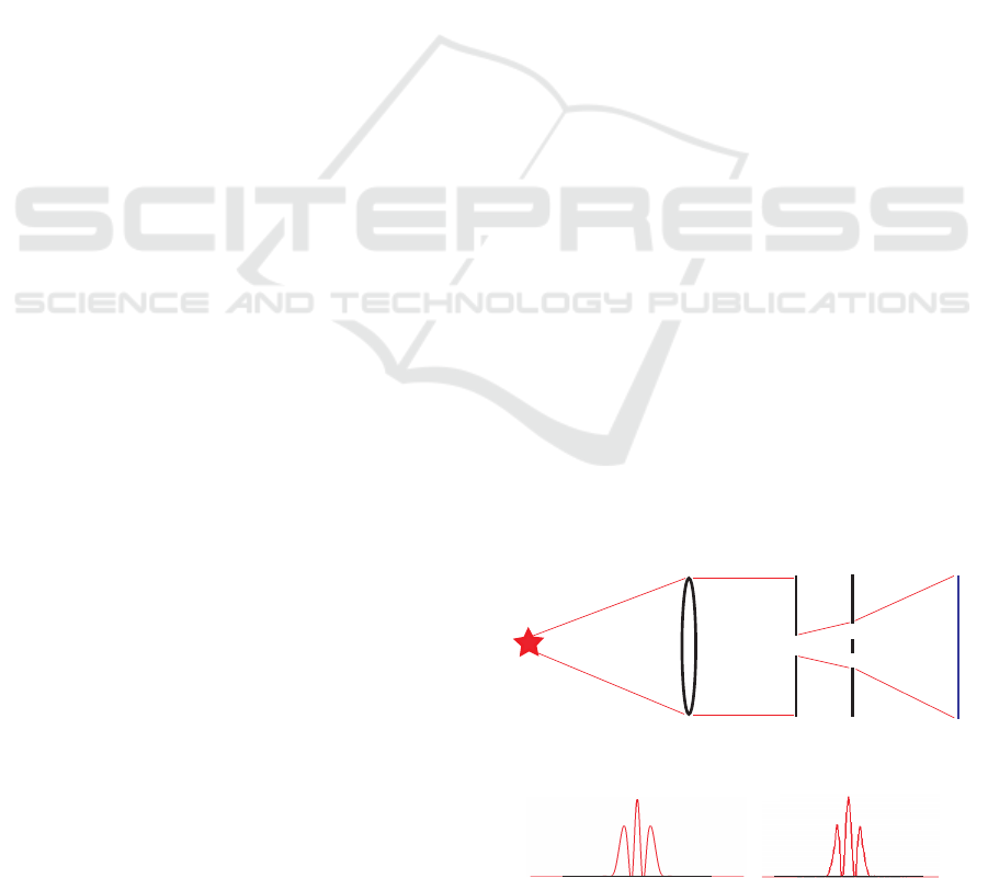
Light Source

Lense

Rectangular

aperture

Slits

Sensor

Naive:28s

Our method:170ms

Conﬁguration

PSF

Figure 1: We present an point spread function simulation of

light passing through a set of lenses and gratings. (Top) An

example conﬁguration of a lens system with several masks

creating a diffraction pattern on the sensor. (Bottom) The

point spread function calculated using simpel phase track-

ing and our speed optimized method.

fects become more prominent. For instance, designs

based on wavefront coding (Dowski and Cathey, ;

Cuypers T., Mertens T., Bekaert P., Baek Oh S. and Raskar R..

INTERACTIVE POINT SPREAD FUNCTION SIMULATION WITH DIFFRACTION AND INTERFERENCE EFFECTS.

DOI: 10.5220/0003379000190024

In Proceedings of the International Conference on Imaging Theory and Applications and International Conference on Information Visualization Theory

and Applications (IMAGAPP-2011), pages 19-24

ISBN: 978-989-8425-46-1

 2011 SCITEPRESS (Science and Technology Publications, Lda.)

Horstmeyer et al., 2010; Schechner et al., 1996) will

demand diffraction and interference. A typical ap-

plication example is a lens with a depth-independent

PSF.

Diffraction and interference effects are governed

by laws from wave optics rather than geometric op-

tics. This increases the implementation complexity

but also the computation time of the simulation. The

latter is not desirable when multiple iterations are re-

quired to ﬁnd the optimal positions for each mask.

The Wigner distribution function (Wigner, 1932) is

a popular light representation and is applicable for

diffraction and interference simulations in the op-

tics community. It basically models light transport

through a grating as a mathematical operation, and

can be applied in a successive fashion for multiple

gratings. The Wigner distribution function is de-

ﬁned in the space–spatial frequency domain which

has recently been shown to have similar properties as

the space–angle domain of the light ﬁeld representa-

tion (Zhang and Levoy, 2009; Oh et al., 2010). Oh et

al (Oh et al., 2010) demonstrated this idea to render

interference patterns. This technique is valid in both

close or far range (near-ﬁeld and far-ﬁeld), however it

is a slow process as it relies on brute-force ray tracing.

We propose a Monte Carlo-based simulation tech-

nique for the Wigner distribution function. As these

calculations are easy to perform in parallel, a GPU

implementation is presented. We show an example

conﬁguration and corresponding PSF on Figure 1 and

show the calculation speed–up compared to the naive

calculation. The resulting computation is in the order

of a fraction of a second, thereby enabling the user

to interactively manipulate the optical conﬁguration

or the projection plane. The proposed method can be

scaled down in precision in order to achieve real-time

performance.

2 RELATED WORK

Light is often described as an electromagnetic ﬁeld

with amplitude and phase. The Huygens–Fresnel

principle is often used to represent wave propagation,

which is a convolution of point scatterers (Goodman,

2005). In contrast, geometrical optics treats light as

a collection of rays. Among the extensive efforts to

connect wave and ray optics (Wolf, 1978), the no-

table ones are the generalized radiance proposed by

Walther (Walther, 1973) and the Wigner Distribution

Function (Bastiaans, 1977; Bastiaans, 1981; Basti-

aans, 1979), where light is described in terms of lo-

cal spatial frequency, which has a simple relationship

with the angular domain. Although the generalized

radiance or the WDF can be negative, they exhibit

convenient properties and explain diffraction rigor-

ously and conveniently (Bastiaans, 1997). We pre-

fer this light representation as it allows us to create

a probability function in space and spatial frequency

for a more efﬁcient Monte Carlo sampling.

In computer graphics, light simulation often in-

volves solving the rendering equation (Kajiya, 1986)

that describes the light propagation. Multiple tech-

niques have been proposed to render wave phenom-

ena in computer graphics. Moravec proposed a

wave model to render complex light transport efﬁ-

ciently (Moravec, 1981), which is based on phase

tracking. This technique keeps track of the travel dis-

tance of a ray and calculates its phase. Ziegler et al.

developed a wave–based framework (Ziegler et al.,

2008), where complex values can be assigned for oc-

cluders to account for phase effects. They also imple-

mented hologram rendering based on wave propaga-

tion (with the spatial frequency) (Ziegler et al., 2007).

Stam implemented a diffraction shader based on the

Kirchhoff integral (Stam, 1999) for random or peri-

odic patterns. Unfortunately, this technique assumes

the light source and observer to be at inﬁnity, and

therefore not suitable for our system.

3 WIGNER DISTRIBUTION

FUNCTION

The Wigner distribution function is a representation

of light commonly used in the optics community. It

is used to simulate of light in both near–ﬁeld and far–

ﬁeld provided that the paraxial approximation is valid.

This approximation assumes that the incoming light

direction is close to the normal direction. For the pur-

pose of plane to plane propagation of light, this as-

sumption is valid.

The microstructure geometry of a diffracting sur-

face can be represented as a complex function t(x) in

space. The amplitude a(x) of t(x) is the amount of

light passing through at position x. The phase part

φ(x) of t(x) represents the phase delay introduced to

the light due to the thickness(height proﬁle) and/or

the refractive index of the surface. We can calculate

the Wigner distribution function (Wigner, 1932) of the

microstructure as

W (x,u) =



x +



∗



x −



−i2πx

(1)

where x is the position, u the spatial frequency and

∗

is the complex conjugate operator. As an incoming

wavefront parallel with the diffracting surface is dis-

torted due to the phase delay, the outgoing wave front

IMAGAPP 2011 - International Conference on Imaging Theory and Applications

a(x)

positive

negative

Figure 2: The Wigner distribution function of an aperture.

(Top) The aperture has an amplitude function which is 1

where the light is passing and 0 elsewhere. (Bottom) The

Wigner distribution of this aperture calculated using Eq 1.

is represented using the same equation in position and

spatial frequency. An example is shown on Figure 2.

The spatial frequency contains the directional in-

formation of a wavefront. There is a simple relation-

ship with the propagation direction θ:

u = sin(θ)/λ (2)

where λ is the wavelength of the light. The basic

concept of the Wigner distribution function is to de-

compose the correlation function of a complex wave-

front into a set of local plane wavefronts with differ-

ent starting positions and spatial frequencies. The in-

tensity of each local plane wavefront is a real value,

which could be negative as well.

3.1 Properties

In order to simulate light propagating through a sys-

tem of lenses and gratings we need a few additional

operators of the Wigner distribution function:

Propagation through Mid–air. The Wigner distri-

bution function W

(x,u) of a complex wavefront will

shear due to the traveling distance z, similar to the

light ﬁeld.

(x,u) = W (x − λuz,u) (3)

Propagation through a Grating. The Wigner dis-

tribution function W

of an outgoing wavefront is a

convolution in spatial frequency of the Wigner distri-

bution function of an incoming wavefront W

and the

Wigner distribution function of the grating W :

(x,u) =

(x,u

− u)W (x,u

)du

(4)

I(x)

p (x)

Projection along u:

p(x , u)

W(x , u)

positive

negative

W(x,u)

Figure 3: Schematic overview of the calculation of p

and

p. (a) The Wigner distribution function of the wavefront in

position–spatial frequency (b) The projection of the wave-

front along u is used to calculate p

, we

construct p(x

,u) using the absolute values of W (x

,u).

Projection on a Surface. The measured intensity

when the light hits a surface such as a camera sensor

is the projection along all spatial frequencies u

I(x) =

W (x,u)du (5)

Even though the Wigner distribution function con-

tains possible negative values, the observed intensity

I(x) on a surface is always positive (Bastiaans, 1997).

3.2 Monte Carlo Simulation

In order to speed up these calculations, we want to nu-

merically estimate the PSF using Monte Carlo simu-

lations. As a simple example, we show the projection

of our wavefront on a plane:

I(x) =

W (x,u)du (6)

≈ (u

min

− u

max

)

∑

i=1

s(x,a) (7)

where s is a sample contributing to the PSF at position

x. This sample is calculated as

s(x,a) = W (x,a)p(x,a) (8)

Which states that we can randomly sample a spatial

frequency a at a position x in the wavefront and add

this value to the total intensity I at position x. The

function p deﬁnes the probability of selecting this

spatial frequency and is added for normalization. In a

case where we uniformly sample a is

p(x,a) =

(9)

with N the amount of samples. This however is sim-

ilar to phase tracking as we select N different paths

thoughout the optical elements.

Alternatively, we can efﬁciently sample I(x) by

selecting our spatial frequency samples (a) according

to its probability function (p). If we sample a within

INTERACTIVE POINT SPREAD FUNCTION SIMULATION WITH DIFFRACTION AND INTERFERENCE

EFFECTS

p (x )

p(x ,u )

x ~

u ~

1 1

p(x ,u - u )

u ~

positive

negative

2 2

x = x -λu z

Figure 4: An overview of the Monte Carlo simulation of

the point spread function. An initial random position and

spatial frequency is sampled according to p

and p. With

each additional grating, a new outgoing spatial frequency

is sampled until it reaches the ﬁnal plane. The intensity of

the sample is calculated based upon the Wigner distribution

function of each grating.

a range of [u

min

max

], the probability function is cal-

culated as

p(x,u) =

min

|W(x,a)|da

max

min

|W(x,a)|da

. (10)

This is not possible with phase tracking as the

importance of a direction is unknown. An example is

demonstrated on Figure 3(a)(c).

When the wavefront has to propagate through

space before it gets projected we have to include the

traveling distance of the light z and a sample is can

therefore be calculated as

s(x + λzu) = W (x, a)p(x, a) (11)

We can solve this by forward propagation, this in-

volves choosing a random start position x

and sample

the spatial frequency u

according to p. This sample

will deﬁne a position x after a propagation distance

z and is added to I(x). Similar to the selective sam-

pling of the spatial frequency we can sample the start

position x

using the probability function

(x) =

min

|W(a,u)|dudx

max

min

|W(a,u)|dudx

. (12)

This function is a also shown on Figure 3(b).

Finally, when a wavefront passes through a grat-

ing, we can also estimate this convolution as

(x,u

) =

W (x,u

− u

(x,u

)du

(13)

≈

∑

i=1

W (x,u

− a)

p(x,u

− a)

(u,a) (14)

Which we simulate by sampling an outgoing spa-

tial frequency u

according to p(x,u). A schematic

overview of this simulation is illustrated in Figure 4.

4 IMPLEMENTATION

Because of the nature of Monte Carlo simulations,

this technique is very suitable for parallel execution.

Therefore we implement part of the algorithm on the

GPU. The implementation can be divided into a pre-

processing step calculating the Wigner distribution

functions and other lookup tables, and rendering step

calculating the diffraction pattern. The implementa-

tion on the CPU is written in C++ for speed and efﬁ-

ciency. The GPU part is implemented using OpenGL

and Cg shaders.

4.1 Pre-processing

We start by calculating a discrete Wigner distribution

function for each diffraction grating micro-structure

t, provided by the user. For example, a rectangular

aperture as shown in Figure 2 has an amplitude func-

tion of a(x) = rect(x/A), where A is the size of the

aperture. We used the fast Fourier transform for an ef-

ﬁcient calculation of the correlation function and the

Fourier decomposition in Eq. (1). This information is

stored into a lookup table in the form of a texture. As

textures are build to hold positive valued intensities,

the positive values of the Wigner distribution function

is stored in the red channel and the negative values in

the green channel.

Having this lookup table also allows precomput-

ing the probability functions p(x, u) and p

(x) as pro-

vided by Eq. (10) and Eq. (12). As we work with a

discrete function, we can easily invert both these func-

tions which we store in the blue and alpha channel of

the texture. This makes sampling of a position and

orientation according to the probability very cheap as

it only requires a single texture lookup.

4.2 Rendering

The rendering consists of N samples which travel

from the ﬁrst grating through the system until they

reach a projection surface. We start by creating these

samples as a set of vertex points in OpenGL. The co-

ordinates of these vertices are randomly chosen be-

tween 0 and 1 as we do not have a function to gener-

ate random values on the GPU. We used the NVidia

Cg library to create a vertex shader that performs the

Monte Carlo simulation based on the random val-

ues provided by the coordinates of the vertex and

the probability function provided by the precomputed

textures.

For each sample, we calculate the position on the

projection screen and translate the sample to this po-

sition in the vertex shader. The intensity is calculated

IMAGAPP 2011 - International Conference on Imaging Theory and Applications

200.000 samples

2 ms

600.000 samples

6 ms

1.000.000 samples

25 ms

4.000.000 samples

90 ms

Ground truth

Figure 5: The amount of samples creates a trade–off between accuracy and speed. Here we show four different renderings of

light passing through a single aperture.

through this path and saved in the red and green

color channels of the vertex similar to the creation

of the textures. These samples are then summed

up using the blend function of the GPU. Due to

the separation of the positive and negative values

of each sample (we can enable the blending using

glBlendFunc(GL ONE,GL ONE)). For precision

we render this process to a 32bit ﬂoating point frame

buffer.

5 RESULTS

The accuracy of the Monte Carlo simulation greatly

depends on the amount of samples we use. This, how-

ever, also increases the calculation speed. Figure 5

shows a comparison between the PSF calculated us-

ing our method and a ground truth of a rectangular

aperture. We notice that by increasing the amount of

samples our results converges to the ground truth.

In the preprocessing step, the lookup–tables are

created and stored into a texture on the GPU. This

step depends on the resolution of the lookup–tables.

To calculate a Wigner distribution lookup table of a

resolution of 1024×1024 and the probability lookup

tables with a resolution of 1024 takes around 800 ms

to calculate on a Intel Core2 6300 – 1.8GHz CPU.

The rest of the result in this section are performed on

an NVidia GeForce 8800 GT.

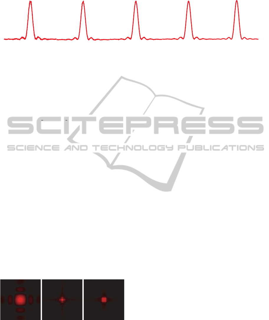
Depth = 15 cm Depth = 7 cm Depth = 1 cm

Figure 6: The Monte Carlo sampling works both in near–

ﬁeld and far–ﬁeld. We show the PSF of a rectangular aper-

ture measured at three different depths. We used 3 million

samples to generate these renderings, which is performed at

80 ms for each rendering.

A speed–up compared to the naive implementation

of the operators of the Wigner distribution function

is presented in Figure 1. The propagation through a

single grating using the naive method requires a com-

putation of 150 ms, which can be reduced to a 15 ms

using our method. Propagating through multiple grat-

ings can reduce the time from 28s to 0.2s.

Finally, we show its applicability in both near–

ﬁeld and far–ﬁeld, which is necessary to construct

PSFs of systems with relative small distance between

the masks. Figure 6 illustrates a PSF of a rectangu-

lar aperture in both near– and far–ﬁeld. The PSF is

calculated in both x and y directions and multiplied to

achieve the presented results.

6 CONCLUSIONS

We presented an efﬁcient implementation for calcu-

lating PSFs using the Wigner distribution function.

Using this representation, we are able to calculate

the diffraction and interference created by small scale

structures of gratings or lenses. Utilizing Monte Carlo

sampling on this function, we are able to simulate the

PSF at interactive speeds. This allows users to inter-

actively adjust parameters.

6.1 Future Work

We demonstrate the calculation of a PSF created by a

1D or 2D gratings which are separable in the 2 dimen-

sions. Extending the theory to a full 2D gratings is

straight forward, but requires a large amount of mem-

ory as the Wigner distribution becomes a function of

4D variables. In order to cope with the limited mem-

ory, we require an intelligent compression method for

data.

ACKNOWLEDGEMENTS

The authors (Tom Cuypers, Tom Mertens and

Philippe Bekaert) acknowledge ﬁnancial support by

INTERACTIVE POINT SPREAD FUNCTION SIMULATION WITH DIFFRACTION AND INTERFERENCE

EFFECTS

the ERDF (European Regional Development Fund),

the European Commission (FP7 IP 2020 3D media)

and the Flemish government. Furthermore, we would

like to thank our colleagues and reviewers for their

useful comments and suggestions.

REFERENCES

Bastiaans, M. (1997). Application of the wigner distribu-

tion function in optics. In The Wigner Distribution -

Theory and Applications in Signal Processing, pages

1227–1238. OSA.

Bastiaans, M. J. (1977). Frequency-Domain Treatment of

Partial Coherence. Optica Acta, 24(3):261–274.

Bastiaans, M. J. (1979). Wigner Distribution Function and

Its Application to 1st-order Optics. J. Opt. Soc. Am.,

pages 1710–1716.

Bastiaans, M. J. (1981). The Wigner Distribution Function

of Partially Coherent-Light. Optica Acta, pages 1227–

1238.

Dowski, E. R. and Cathey, W. T. Extended Depth of Field

through Wave-Front Coding. Applied Optics.

Goodman, J. W. (2005). Introduction to Fourier optics.

Roberts & Co., Englewood, Colo., 3rd edition.

Horstmeyer, R., Oh, S. B., and Raskar, R. (2010). Itera-

tive aperture mask design in phase space using a rank

constraint. Opt. Express.

Kajiya, J. T. (1986). The rendering equation. In Pro-

ceedings of the 13th annual conference on Computer

graphics and interactive techniques, SIGGRAPH ’86,

pages 143–150, New York, NY, USA. ACM.

Moravec, H. P. (1981). 3d graphics and the wave the-

ory. In Proceedings of the 8th annual conference on

Computer graphics and interactive techniques, SIG-

GRAPH ’81, pages 289–296, NY, USA. ACM.

Oh, S. B., Kashyap, S., Garg, R., Chandran, S., and Raskar,

R. (2010). Rendering wave effects with augmented

light ﬁelds. EuroGraphics.

Schechner, Y. Y., Piestun, R., and Shamir, J. (1996).

Wave propagation with rotating intensity distribu-

tions. Phys. Rev. E.

Stam, J. (1999). Diffraction shaders. In Proceedings of

the 26th annual conference on Computer graphics

and interactive techniques, SIGGRAPH ’99, pages

101–110, New York, NY, USA. ACM Press/Addison-

Wesley Publishing Co.

Walther, A. (1973). Radiometry and Coherence. J. Opt Soc.

Am.

Wigner, E. (1932). On the quantum correction for thermo-

dynamic equilibrium. Physical Review.

Wolf, E. (1978). Coherence and Radiometry. Journal of

Optical Society of America.

Zhang, Z. and Levoy, M. (2009). Wigner distributions and

how they relate to the light ﬁeld. In IEEE ICCP.

Ziegler, R., Bucheli, S., Ahrenberg, L., Magnor, M., and

Gross, M. (2007). A bidirectional light ﬁeld - holo-

gram transform. Comp. Gr. Forum.

Ziegler, R., Croci, S., and Gross, M. H. (2008). Lighting

and occlusion in a wave-based framework. Computer

Graphics Forum.

IMAGAPP 2011 - International Conference on Imaging Theory and Applications