
DYNAMIC OBSTACLE AVOIDANCE FOR AN ACKERMAN
VEHICLE
A Vector Field Approach
Tommie Liddy, Tien-Fu Lu
School of Mechanical Engineering, The University of Adelaide, SA 5005, Adelaide, Australia
David Harvey
Aerospace Concepts, 17 Yallourn St, ACT 2609, Fyshwick, Australia
Keywords: Autonomous navigation, Vector field, Obstacle avoidance, Ackerman vehicle, AGV.
Abstract: A vector field navigation system was shown to avoid dynamic obstacles and reach a goal with a pre-
specified position and heading using a simulated Ackerman vehicle. The navigation system was divided
into two distinct vector fields, an environmental field which was created for goal oriented navigation and
obstacle field which was designed for obstacle avoidance. Discussed in this paper were the methods of
obstacle avoidance and combining the two fields of the navigation system. The obstacle avoidance method
created a rotational vector field centred on a single obstacle. Algorithms were created to select the obstacle
that would be the centre of the field and the direction of rotation of the field. A parameter based method
was used to combine the obstacle field and the environmental field. A simulation workspace was created to
show the navigation behaviours created by combining these methods and a sample of these results were
presented in this paper.
1 INTRODUCTION
The use of vector fields can be a simple and
mathematically low cost method of both navigation
and obstacle avoidance for an autonomous vehicle
(Borenstein, 1989). Many methods use multiple
vector fields to produce a navigation strategy. The
typical form of this approach is to have one vector
field represent the desired motion of an unobstructed
vehicle and another represent the motion required
for obstacle avoidance (Xiao 1998; Ge, 2002; Lui,
2006). These vectors are than added together to
achieve all navigation goals. This method can
produce a local minimum which will effectively stop
a vehicle from reaching its goal and the unstable
movement of a vehicle (Koren 1991; Lui 2006).
There are methods that produce a single field
acting to avoid obstacles and reach a desired goal
(Kim, 1999; Loizou 2003; Lindermann 2006).
These approaches offer benefits such as smother
travel but rely on prior knowledge to create the field.
If no prior knowledge of obstacles and navigational
boundaries are available these methods cannot be
applied to a real time dynamic environment.
Through this paper a navigation system will be
introduced that allows an autonomous vehicle to
avoid dynamic obstacles in real time. A multiple
vector field approach was taken to create this
navigation system. An Environmental vector was
created using a method outlined in Liddy 2007. An
obsrtacle vector was created using the configuration
of the obstacles the mobile platform had detected as
well as the relative vehicle and waypoint positions.
A method described for combining these two vector
fields will also be shown, building apon the
algorithms presented in Liddy 2008.
The results presented in this paper will show that
this method was able to produce a navigation
strategy allowing an Ackermann vehicle to
successfully navigate a dynamic scenario. The
inherant limitations of the system will also be
examined. Primarily the ability of the navigation
method to cope with obstacles moving at roughly the
same speed as the vehicle.
93
Liddy T., Lu T. and Harvey D..
DYNAMIC OBSTACLE AVOIDANCE FOR AN ACKERMAN VEHICLE - A Vector Field Approach.
DOI: 10.5220/0003383100930098
In Proceedings of the 8th International Conference on Informatics in Control, Automation and Robotics (ICINCO-2011), pages 93-98
ISBN: 978-989-8425-75-1
Copyright
c
2011 SCITEPRESS (Science and Technology Publications, Lda.)
2 SIMULATION ENVIRONMENT
Experiments were conducted in a simulated
environment. A mathematical model (Liddy, 2007,
Hashim, 2009) was used to represent the mobile
platform with dimensions shown in Table 1 and
Figure 1. The environment in which the simulated
vehicle travelled was considered flat in the X-Y
plane. Waypoints were used as navigational
markers and consisted of a position in the X-Y plane
and a heading
()
WPWPWP
yx
θ
,, . Each obstacle
consisting of a array of positions in the X-Y plane, a
length and width along the x and y axis and a
velocity
()
OBOBOBOBOB
vwlyx ,,,
~
,
~
. An obstacle
would move from one point in the position array to
the next at v
ob
. For simplicity the obstacles were all
made to have the same dimensions for all tests
(l
OB
=310mm w
OB
=400mm) and the velocity of all
obstacles was set to the same value for each
individual test.
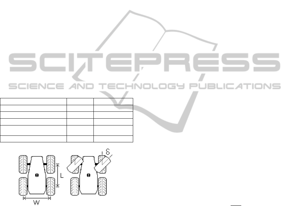
Table 1: Vehicle dimensions and properties.
Property Symbol Value
Vehicle length L 300mm
Vehicle width W 300mm
Maximum steering angle δ 25˚
Maximum steering rate
δ
30˚/sec
Vehicle velocity V 1000mm/sec
Figure 1: Dimensions of the simulated vehicle.
A sensor model was also employed to simulate
the ability of the mobile platform to detect obstacles.
The model was designed to sort the obstacles present
in the navigation environment as either visible or not
visible. An ideal model of a planar laser scanner
was used to achieve this. The model was given a
sensor range of 3000mm (D
SEN
=3000mm) and a
sensor angle of ±90˚ from the vehicle’s X-axis
(θ
SEN
=90˚). These characteristics (D
SEN
and θ
SEN
)
were used to form a visible region in front of the
vehicle. All obstacles in that region were considered
to be detectable and were made visible to the mobile
platform. This included any dynamic obstacle,
however information regarding their trajectory was
not made known the mobile platform. The mobile
platform stored the last known position of obstacles
when they were no longer in the visible region. The
obstacles were assumed to remain in that position
unless that space was shown to be clear.
The simulation tests were run as real time
navigational scenarios. The position of the vehicle
and dynamic obstacles were updated at 250ms
intervals. The mobile platform was given no prior
knowledge of the obstacles in the environment only
a starting position and waypoint. Each test was
initialised with the vehicle at a position of (0mm,
0mm) with a heading of 0˚. The criteria for
completing a test were that the vehicle must be
within 1000mm of the goal and be moving away
from said goal.
3 OBSTACLE VECTOR FIELD
The objective of the obstacle vector field was to
produce a force which acted on the mobile platform
in such a way that caused it to avoid an obstacle.
The blend function, the obstacle field rotational
direction and the pivot block determine the
characteristics of the navigation system (Liddy et al.,
2008).
3.1 Blend Function
The blend function producd a weighting value which
acted to combine the environmental vector field
(E
VF
) and the obstacle vector field (O
VF
) into the
navigational vector field (N
VF
) as shown in
Equations (1), (2) and (3).
⎟
⎟
⎠
⎞
⎜
⎜
⎝
⎛
⎟
⎟
⎠
⎞
⎜
⎜
⎝
⎛
⎟
⎟
⎠
⎞
⎜
⎜
⎝
⎛
+= 1,0,maxmin
xi
i
iii
N
x
OFFSBf
(1)
()
∏
⇒
⇒
−−=
i
m
im
BfBf
1
1
11
(2)
(
)
VFmVFmVF
OBfEBfN *1*
11 ⇒⇒
−
+
=
(3)
Each blend function used a single parameter
from the navigation system (x
i
) with three constants
selected to shape the function (N
xi
, OFF
i
and S
i
).
The constant N
xi
was used to normalise the
navigation variable. The OFF
i
constant was used to
offset the function, specifically to select the point
where Bf
i
becomes greater than zero. S
i
was used to
control the slope of Bf
i
which, with the use of OFF
i
was used to select the point where Bf
i
became equal
ICINCO 2011 - 8th International Conference on Informatics in Control, Automation and Robotics
94
to one. Each blend function was created to address
scenarios in which obstacle avoidance would be
desired
For a real time navigation system it was seen that
obstacle avoidance behaviours would be required
when an obstacle was in front of a vehicle or close to
a vehicle. To address this two blend functions were
created as shown in Table 2.
Table 2: Blend function parameters.
x
i
N
xi
OFF
i
S
i
The minimum distance
between any obstacle and
the mobile platform.
3000mm -0.25 2
The minimum absolute
angle created between any
obstacle, the mobile
platform and the waypoint
2
π
-0.25 2
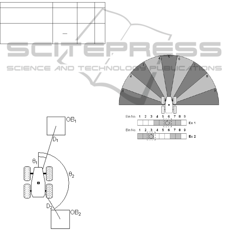
3.2 Pivot Block
The pivot block was the obstacle selected as the
centre of the obstacle vector field. This obstacle was
selected based the obstacle position relative to the
vehicle. The pivot block was classified as the
nearest known obstacle located in front of the
vehicle. The example shown in Figure 2 would have
OB
1
as the pivot block even if D
2
<D
1
because OB
2
would be considered to be behind the vehicle
(θ
2
>90˚).
Figure 2: Selection of the pivot blot, example.
3.3 Obstacle Vector Field Rotational
Direction
A vector was produced at an obstacle as a rotational
field. Navigation behaviours were developed by
basing the direction of rotation of that field on
various parameters. These behaviours could be
summarised as follows, if the vehicle was
confronted by an obstacle it was required to move
around it on what was considered the clearer side.
This was done by selecting the rotational direction
that required the vehicle turn as little as possible.
To implement this behaviour a angled histogram
was used to determine where free space was and
where obstacles blocked the immediate path. An
angle bin of 20˚ was selected and the histogram was
created over 180˚ (±90˚ from the vehicle X-axis). If
any known obstacle occupied a particular bin that
bin was set to one, otherwise it was set to zero.
Figure 3: The angled histogram with 9 bins of 20˚;
Example 1 shows the histogram when there are obstacles
clustered to the right and directly in front of the vehicle;
Example 2 shows the histogram when there are obstacle to
either side of the vehicle.
A graphical representation of the histogram is
shown in Figure 3 with two examples representing
states which could occur during run time. In the
examples shown in this figure a grey box
represented a bin was set to one and the dotted
outlined indicated the bin that contained the pivot
block. The rotational direction was selected based
on two parameters. The closest unoccupied bin to
the central bin in the histogram, and the bin
containing the pivot block. If the bin containing the
pivot block was higher than the closest unoccupied
bin to the centre the rotation direction was clockwise
(Example 1) and if the opposite was true it was anti-
clockwise (Example 2).
DYNAMIC OBSTACLE AVOIDANCE FOR AN ACKERMAN VEHICLE - A Vector Field Approach
95
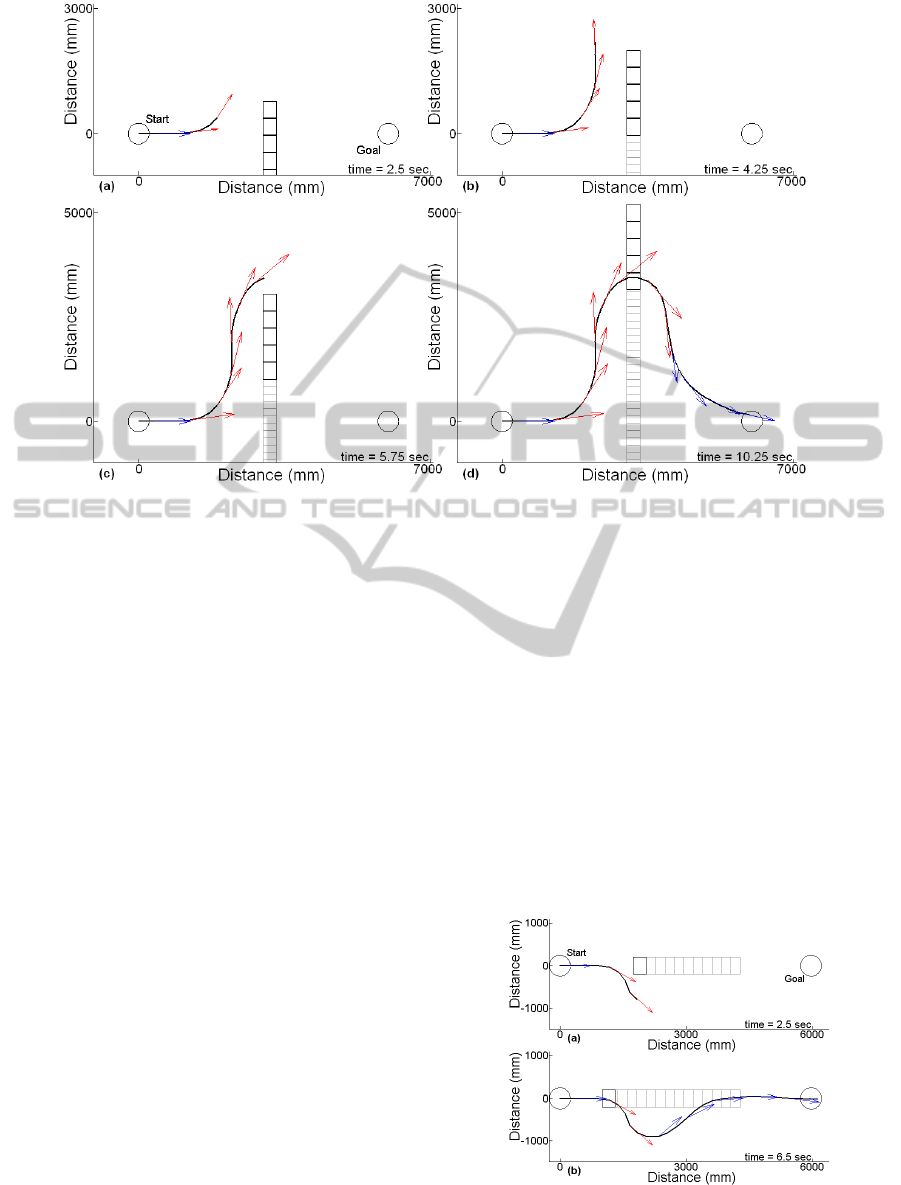
Figure 4: Vehicle avoiding a side on collision with an elongated obstacle with a waypoint at (6000,0,0); V = 1000mm/s;
V
OB
= 700mm/s: (a) time = 2.5 sec (b) time = 4.25 sec (c) time = 5.75 sec (d) time = 10.25 sec.
4 RESULTS
A series of experiments were run to show the
capabilities of the combined navigation and obstacle
avoidance methods discussed in Liddy et al. 2007;
2008 when applied to a dynamic environment.
Experiments were run on a simulation platform
under real time conditions. Initial tests focused on
the possible limitations of dynamic obstacle
avoidance with regards to vehicle and obstacle
relative speeds (Section 4.1). Further results show
the navigation traits when acting within those
limitations (Section 4.2). All results show the
vehicle and obstacle paths up to a specified time.
The desired navigation vector was attached to the
vehicle’s path at regular intervals. A blue vector
represents a blend factor of one, whereas a red
vector represents a blend factor between one and
zero.
4.1 Navigation Limitations
The tests shown in Figure 4 and 5 illustrate scenarios
where comparative speed between vehicle and
obstacle were an issue. The possibility of a side on
collision and a head on collision were examined in
these scenarios.
Under a specific condition a side on collision was
found to be unavoidable. For this collision to occur
the vehicle must initially encounter the obstacle
when a large portion of the obstacle was on the side
of the vehicle the obstacle was coming from. This
configuration was met when the vehicle encountered
the obstacle as shown in Figure 4 (a). At this point it
can be seen that the navigation algorithm steered the
vehicle around the obstacle in the direction the
obstacle was moving. Figure 4 (b) and (c) show that
the vehicle moved parallel to the obstacle and then
attempted to pass in front of the obstacle’s path.
This motion allowed the obstacle to close the
distance to the vehicle. It was found that an obstacle
speed approximately 70% of that of the vehicle was
the maximum allowable without a collision
Figure 5: Vehicle avoiding a head on collision with a
single obstacle, waypoint at (6000,0,0); V = 1000 mm/s;
V
OB
= 900 mm/s: (a) time = 2.5 sec (b) time = 6.5 sec.
ICINCO 2011 - 8th International Conference on Informatics in Control, Automation and Robotics
96
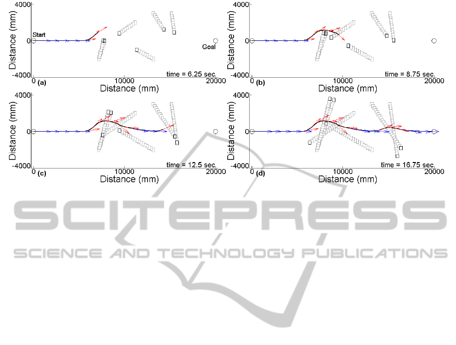
Figure 6: Vehicle avoiding multiple obstacles in a sparsely cluttered environment with a waypoint at (20000,0,0);
V = 1000mm/s; V
OB
= 350mm/s: (a) time = 6.25 sec (b) time = 8.75 sec (c) time = 12.5 sec (d) time = 16.75 sec.
The scenario presented in Figure 5 shows
another situation where a collision was likely to
occur. The limiting factors for this scenario were the
speeds of both the vehicle and the obstacle and the
visible distance the sensor model allowed for
obstacle detection. Essentially, the mobile platform
was required to move out of the way of the obstacle
in the time between when it identified the obstacle
and when the obstacle would close the distance to
the vehicle. Results shown indicate the maximum
speed of a single obstacle where collision did not
occur was 900mm/s as shown in Figure 5. For
larger obstacles this value would be diminished.
4.2 Dynamic Obstacle Avoidance
To examine the behaviour of the navigation
algorithm the mobile platform was placed in several
scenarios which involved multiple static and
dynamic obstacles. All dynamic obstacles were set
to move at the same speed (350 mm/s). This speed
was within the maximums obtained while analysing
the obstacle avoidance limitations (Section 4.1).
The results obtained in doing so showed the traits
inherent in the navigation method.
A scenario was run showing the mobile platform
passing through an area populated with
independently moving obstacles, shown in Figure 6.
In this scenario the vehicle initially moved directly
towards the waypoint until it encountered a set of
obstacles at 6.25 seconds, shown in Figure 6 (a). At
this instance it can be seen from the red vectors
present that the obstacle avoidance algorithm began
to influence navigation. The algorithm steered the
mobile platform to the clearer side of the area the
sensor system could see. This behaviour was
repeated a second time at 12.5 seconds, shown in
Figure 6 (c). Although in one instance the vehicle
moved in front of the obstacle and in the other it
moved behind this behaviour was still consistent
when viewed through the navigation algorithm.
While avoiding one set of obstacles the mobile
platform encountered a second set, this can be seen
in Figure 6 (b). This second encounter elongated the
duration the obstacle vector field had control of the
vehicle. During that period the pivot block was
required to switch between the four obstacles
present. The obstacle vector field and blend factor
were altered with each switch ensuring the mobile
platform avoided all obstacles.
The example presented in Figure 7 shows the ability
of the navigation system to identify gaps and steer
the vehicle through them. In Figure 7 (a) it can be
seen that the vehicle encountered a dynamic obstacle
while avoiding a set of static obstacles. The vehicle
was forced towards the dynamic obstacle due to the
structure of the static obstacles. At this point the
vehicle was able to identify a gap between the
obstacles and steer the vehicle towards it. This
behaviour indicated that when there was sufficient
space available the vehicle would pass through a gap
if it were the best option available. This behaviour
can be seen again between the 6 and 8.25 second
mark, Figure 7 (b) and (c), as the vehicle passed
between a static wall of obstacles and a dynamic
obstacle. In both instances the gap was selected
because it would lead the vehicle into clear space
and away from the obstacles directly in front of it.
DYNAMIC OBSTACLE AVOIDANCE FOR AN ACKERMAN VEHICLE - A Vector Field Approach
97
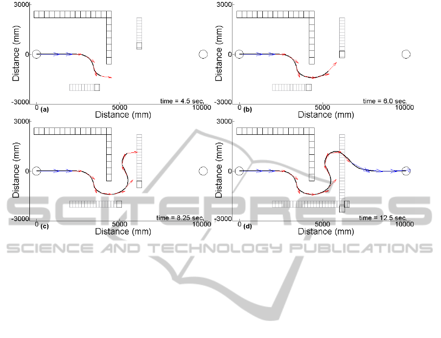
Figure 7: Vehicle static and dynamic obstacles in a structured environment with a waypoint at (10000,0,0);
V = 1000mm/s; V
OB
= 350mm/s: (a) time = 4.5 sec (b) time = 6.0 sec (c) time = 8.25 sec (d) time = 12.5 sec.
5 CONCLUSIONS
Presented in this paper was a navigation algorithm
developed to operate in a dynamic environment. A
method was outlined showing the use of a blend
function and pivot block (defined in Sections 3.1 and
3.2) with an existing method of vector creation to
produce a navigation algorithm. Results gathered
using this method were shown to have measurable
limitations under specific circumstances. When
operated within these limitations the navigation
algorithm was shown to be able to safely control a
mobile platform in a dynamic environment.
REFERENCES
J. Borenstein and Y. Koren. Real-Time Obstacle
Avoidance for Fast Mobile Robots. IEEE Transactions
on Systems, Man, and Cybernetics. Vol. 19 pp. 1179-
1187, 1989.
Dongbo Xiao and Roger Hubbold. “Navigation guided by
artificial force fields”, SIGCHI Conference on Human
factors in computing systems, China, 1998.
S. S. Ge and Y. J. Cui, "Dynamic Motion Planning for
Mobile Robots Using Potential Field Method",
Autonomous Robots, vol 13 pp 207-222, 2002.
D. K. Lui, D. Wang and G. Dissanayake, “A Force Field
Method Based Multi-Robot Collaboration”, IEEE
Conference on Robotics, Automation and
Mechatronics, 2006.
Koren and Borenstein, “Potential Field Methods and their
Inherent Limitations for Mobile Robot Navigation”,
IEEE Conference on Robotics and Automation, 1991.
Yong-Jae Kim, Dong-Han Kim and Jong-Hwan Kim.
“Evolutionary Programming-Based Uni-vector Field
Method for Fast Mobile Robot Navigation”. SEAL’98,
LNCS 1585, pp. 154-161, 1999.
Savvas G. Loizou, Herbert G. Tanner, Vijay Kumar and
Kostas J. Kyriakopoulos. “Closed Loop Motion
Planning and Control for Mobile Robots in Uncertain
Environments”. IEEE Conference on Decision and
Control, Vol. 3, pp. 2926-2931, 2003.
Stephen R. Lindemann, Islam I. Hussein and Steven M.
LaValle, “Real Time Feedback Control for
Nonholonomic Mobile Robots With Obstacles”, IEEE
Conference on Decision and Control, 2006.
Tommie Liddy and Tien-Fu Lu, “Waypoint Navigation
with Position and Heading Control using Complex
Vector Fields for an Ackermann Steering Autonomous
Vehicle”, Australasian Conference on Robotics and
Automation, 2007.
Tommie Liddy, Tien-Fu Lu, Peter Lozo and David
Harvey, “Obstacle Avoidance Using Complex Vector
Fields”. Australasian Conference on Robotics and
Automation, 2008
Sani Hashim and Tien-Fu Lu, “A new strategy in dynamic
time-dependent motion planning for nonholonomic
mobile robots”, 2009 IEEE International Conference
on Robotics and Biomimetics, China, 2009.
ICINCO 2011 - 8th International Conference on Informatics in Control, Automation and Robotics
98
