
SYMMETRY AND STABILITY OF HOMOGENEOUS FLOCKS
J. J. P. Veerman
Fariborz Maseeh Dept of Math. and Stat., Portland State University, Portland, OR 97201, U.S.A.
Keywords:
Coupled oscillators, Network, Stability, Symmetry, Decentralized control.
Abstract:
The study of the movement of flocks, whether biological or technological, is motivated by the desire to under-
stand the capability of coherent motion of a large number of agents that only receive very limited information.
In a biological flock a large group of animals seek their course while moving in a more or less fixed formation.
It seems reasonable that the immediate course is determined by leaders at the boundary of the flock. The oth-
ers follow: what is their algorithm? The most popular technological application consists of cars on a one-lane
road. The light turns green and the lead car accelerates. What is the efficient algorithm for the others to closely
follow without accidents? In this position paper we present some general questions from a more fundamental
point of view. We believe that the time is right to solve many of these questions: they are within our reach.
1 INTRODUCTION
We model agents and their interactions as a finite net-
work of (coupled) oscillators in R
d
. We assume that
agents observe relative positions and velocities only
(no third and higher derivatives). The best studied ex-
ample of such a flock is a class of well-known models
for cars equipped with sensors and on automatic pilot
that are moving in close formation on a one-lane road.
However, we are interested in a wider class of flocks
(especially those moving in R
2
and R
3
). Our main
concerns in this position paper fall in two categories:
- What are the equations we should study?
- What does it mean for a (large) flock to be stable?
These are the questions that motivate this position pa-
per.In our view their will give rise to exciting new
mathematics with ample implications for the sciences.
In response to the first concern we present phys-
ical considerations that impel us to consider transla-
tional symmetry of the equations of motion (in Sec-
tion 2) and rotational symmetry and its breaking (in
Section 3). These considerations are perhaps not
fundamentally new: but the literature favors detailed
studies that are of immediate technological impor-
tance. However, we argue that these equations can
— and should — successfully be attacked.
The second concern is addressed in Section 4.
We’ll see that even in an asymptotically stable sys-
tem, fluctuations may grow very large before they at-
tenuate and die out. In one dimension they lead to
collisions. In dimension greater than one, collisions
are perhaps unlikely, but large fluctuations could lead
to loss of cohesion of the flock (because the agents
can’t “see” each other anymore). Clearly there is a
limit to the size of the fluctuations a flock can sustain.
We will argue that it is useful to study this kind of
stability in the time domain. We also argue that more
general methods to investigate this kind of “transient
(in)stability” should be researched.
We’ll use a very simple set-up of a 1 dimensional
flocks as our ‘standard example’.
Definition 1.1 (Standard Example). Consider N + 1
agents in R labeled from 0 to N, each of whose co-
ordinates are given by z
k
(t) as function of time. For
k ∈ { 1··· , N − 1}, let f and g be negative and ρ and
r are in (0, 1).
¨z
k
= f {z
k
− (1− ρ)z
k−1
− ρz
k+1
}
+g{˙z
k
− (1− r)˙z
k−1
− r˙z
k+1
}
The boundary conditions are:
¨z
0
= 0 and ¨z
N
= f {z
N
− z
N−1
} + g{˙z
N
− ˙z
N−1
}
The initial conditions are:
∀ k : z
k
(0) = 0, ∀ k > 0 : ˙z
k
(0) = −0.1, ˙z
0
(0) = 0.
It should be understood that the original coordinates
of the agents given by x
k
where x
k
= z
k
+ h
k
; those
are the coordinates we display in Figure 2. The {h
k
}
are priori chosen constants and their differences de-
termine the preferred relative positions of the agents.
470
Veerman J..
SYMMETRY AND STABILITY OF HOMOGENEOUS FLOCKS.
DOI: 10.5220/0003400204700475
In Proceedings of the 1st International Conference on Pervasive and Embedded Computing and Communication Systems (PECCS-2011), pages
470-475
ISBN: 978-989-8425-48-5
Copyright
c
2011 SCITEPRESS (Science and Technology Publications, Lda.)

2 TRULY DECENTRALIZED
LINEAR FLOCKS
Ever since the inception ((Chandler et al., 1958),
(Herman et al., 1959)) of the subject it has been a
challenge to mathematically express the notion “de-
centralized” ((Chu, 1974)). Here is how we interpret
it: In a decentralized flock the only information an
agent receives are the position and velocity relative to
it of some nearby agents. The agents do not receive
information from an outside source. The only excep-
tions to this are some agents, called leaders, who may
undergo an external forcing.
Proposition 2.1 (Galilean Invariance). In the ab-
sence of external forcing, the motion of a truly de-
centralized linear flock in R is described by (k and i
in {0· ··N}):
¨x
k
= f
∑
i∈N
ρ
(k)
L
ρ,ki
(x
i
− h
i
) + g
∑
i∈N
r
(k)
L
r,ki
˙x
i
or ¨z
k
= f
∑
i∈N
ρ
(k)
L
ρ,ki
z
i
+ g
∑
i∈N
r
(k)
L
r,ki
˙z
i
.
where z
k
= x
k
− h
k
. The row-sums of the N + 1 by
N + 1 “Laplacian” matrices L
ρ
and L
r
must be zero.
The sums are over the set of agents N
ρ
whose relative
velocity can be measured by k, resp. whose relative
position can be measured by K (in the case of N
r
).
We furthermore have that there is a 2-parameter set
of solutions given by (for any Z and V in R):
∀ k ∈ {0··· , N} : z
k
(t) = Vt + Z .
From now on we will always assume that f and
g are chosen so that the system is asymptotically
stable, that is: in the absence of external forcing,
the system always converges to an orbit of the form
z
k
(t) = Vt + Z. We call such a system stabilized. In
the standard example, the stipulation that f and g be
negative guarantees this. For general Laplacians, and
especially in dimension bigger than 1, it not neces-
sarily obvious how to achieve this and that question
merits more attention.
In the following we denote z ≡ (z
0
··· ,z
N
)
T
in
C
N+1
. Similarly a is in C
N+1
.
Lemma 2.2. Suppose in the system of Proposition 2.1
agent “0” is the only leader and its orbit is given by
z
0
(t) = e
iωt
. Then as t → ∞ the orbit of the system
converges to
z(t) = ae
iωt
,
where Galilean Invariance implies that
a = (a
0
··· ,a
N
) ∈ C
n
satisfies:
−ω
2
a = ( fL
ρ
+ iωgL
r
)a .
And in particular lim
ω→0
a
k
(ω) = 1 for all k ∈
{0·· · ,N}.
This Lemma is immediately relevant to the present
discussion because it indicates that certain low-
frequency perturbations in the orbit of the leader can-
not possibly die out: it is impossible to design a de-
centralized system where all perturbations die out.
The situation is in fact probably worse: as the size of
the system grows, it seems that, say, max
ω∈R
+ |a
N
(ω)|
must also grow, probably with some power 1/d of the
number N of agents, where perhaps d is related to a
notion of the dimensionality of the “communication
graph”. This question has received some attention
((Pant et al., 2002)), but not nearly enough.
The trouble doesn’t even end there. When we
study flocks — whether biological or technological
— it is natural to assume that each agent performs
the same computation to determine its acceleration.
When you imagine a large flock then for all agents
‘sort of’ in the middle of that flock that assumption is
reasonable: all agents are hardwired equal. We’ll call
this homogeneity. It is hard to give a formal definition
of this concept since it cannot be completely true for
a finite flock moving in R
d
: the agents at the physical
boundary of the flock necessarily have less neighbors.
Since perturbations cannot all die out — as we just
showed, the boundary conditions may well influence
the dynamics of the flock. We can see two possibili-
ties: either boundary conditions (or some natural sub-
set thereof) don’t matter, or else there is a smart and
natural way of uniquely specifying them. To the best
of our knowledge this important question has hardly
if ever been addressed (except (Sullivan, 2010), un-
published)!
3 DECENTRALIZED FLOCKS
IN A MEDIUM, MASS
We do not live in a vacuum! Whatever our method
of locomotion is, in a medium we can perceive our
speed with respect to the medium, by the effort we
expend to maintain the speed to overcome friction.
(Though without a compass we cannot measure the
direction of that speed.) The consequence of perceiv-
ing speed is that there is a preferred direction for the
agents, namely: forward (in the direction of the veloc-
ity). Thus flocks in dimension 2 can orient themselves
so that their desired configuration is aligned along the
velocity of the flock.
To formulate those equations in R
2
let’s go back
to the system given in Proposition 2.1 in the coordi-
nates of the agents given by x
k
where x
k
= z
k
+h
k
(the
SYMMETRY AND STABILITY OF HOMOGENEOUS FLOCKS
471

first of the two equations). We now interpret x
k
and
h
k
as vectors in R
2
. These equations are not truly de-
centralized anymore! An agent unsure where North is
can only measure |h
k
− h
k−1
| (ie: relative distances).
However flying in a medium, the agent can perceive
their direction of flight and orient itself according to
it (as long as their speed is non-zero.) Thus the rota-
tional symmetry of the truly decentralized equations
in dimension 2 can be broken. We argue that this is
how geese manage to fly in formation. Here are the
equations:
Proposition 3.1 ((Veerman et al., 2005)). Let θ
k
be
angle that ˙x
k
makes with the positive x-axis. Denote
by R
θ
the rotation by θ. The equation of motion for
the orientable flock is:
¨x
k
= f
∑
i∈N
ρ
(k)
L
ρ,ki
(x
i
− R
θ
k
h
i
) + g
∑
i∈N
r
(k)
L
r,ki
˙x
i
,
as long as all ˙x
i
are non-zero. (The equation has a
singularity at ˙x
i
= 0.)
In Figure 1 taken from (Veerman et al., 2005) we
show a numerical simulation using the Equations of
Proposition 3.1. The figure shows that in principle
it is possible to re-orient a (mathematical) flock as
it turns. (Remark: The way we did it in that paper
is not exactly how we propose to study that ques-
tion here. But it does provide a proof of concept.)
(See also (Williams et al., 2005)) The important ques-
tion is: how can we understand the re-alignment of a
flock in 2 (or 3) dimensions that changes its direction
when certain leaders at its boundary initiate a course
change. We invite the reader to study these equations!
The non-linearity makes these equations a real chal-
lenge to study (a few results are given in (Veerman
et al., 2005)).
This leaves two other questions. It is possible to
introduce a desired speed V in the above equations.
Furthermore in a realistic flock it is likely that the
masses m
k
of the agents have a distribution with aver-
age 1 (as opposed to being exactly 1). The equations
(in the absence of any external forces) then become:
m
k
¨x
k
= f
∑
i∈N
ρ
(k)
L
ρ,ki
(x
i
− R
θ
k
h
i
)+
g
∑
i∈N
r
(k)
L
r,ki
˙x
i
+ α
1−
V
| ˙x
k
|
˙x
k
.
(1)
Here α < 0. We expect that both the presence of de-
sired speed (a cruise speed) and the variation in the
masses act to stabilize the equations to some extent.
In a realistic setting we probably want flocks to be
able to travel at different speeds: in different envi-
ronments (say, cities or freeways) the desired cruise
speeds should be different. Furthermore even when
we agree on a single desired cruise speed, it appears
unrealistic that individual agents in dense traffic can
−200 −100 0 100 200 300 400 500 600
0
100
200
300
400
500
600
Figure 1: (color online) This figure is a simulation of a flock
turning around using Definition 3.1. Note that the orienta-
tion of the flock’s configuration changes. Each ‘Christmas
tree’ shaped hexagon is a snapshot of the position of the
flock, the lines that form the figure only facilitate visual in-
spection, they have no physical or mathematical content.
be programmed to determine their absolute speed ac-
curately enough so as to avoid collisions with their
immediate neighbors. Nonetheless we offer Equation
1 as a possible starting point for a more general math-
ematical study of flocking in 2 dimensions than the
equation in Proposition 3.1.
4 SYMMETRY AND STABILITY
Now we come to what is certainly one of the most
intriguing and important questions concerning flocks:
What happens if a member at the “boundary” of the
flock suddenly its velocity for whatever reason (a
predator is observed or a traffic light changes etc)?
How is the capability of following the new — sup-
posedly more advantageous — affected by the size
of the flock? The (in)ability to effectively follow the
new course should limit the maximum allowable size
of the flock. What is that size, and how can we imple-
ment that in a ‘technological’ flock? Recall that we
assume that a flock is asymptotically stable, so that
no matter what the course change is, the other agents
will ultimately follow the leader. The catch is that if,
prior to stabilizing, fluctuations become too large: the
flock is still not viable. Sometimes this is informally
referred to as ‘transient stability’. In the literature the
concept of ‘string stability’ has played an important
role ((Swaroop and Hedrick, 1996a), (Swaroop and
Hedrick, 1996b)).
Let’s look at the Standard Example (Definition
1.1). That system is given in such a way that
lim
t→∞
z(t) = 0 and lim
t→∞
˙z(t) = 0. This is im-
PECCS 2011 - International Conference on Pervasive and Embedded Computing and Communication Systems
472

portant in what follows. Consider the quantities
max
k
max
ω≥0
|a
k
(ω)| and of max
k
max
t≥0
|z
k
(t)|. It
turns out that the maxima are achieved for k = N,
which simplifies the notation.
Definition 4.1. We call the system ‘harmonically un-
stable’ if
1
N
lnmax
ω≥0
|a
N
(ω)| > 0 ,
and ‘impulse unstable’ if
1
N
lnmax
t≥0
|z
N
(t)| > 0 .
The system is ‘flock unstable’ if either holds, ‘flock
stable’ otherwise.
Theorem 4.2 ((Veerman et al., 2009), (Veerman,
2010), (Veerman and Tangerman, 2010), (Tanger-
man et al., 2010)). The system given in Definition
1.1 with r = ρ is harmonically and impulse stable
ρ = 1/2 and harmonically and impulse unstable for
ρ ∈ (0,1)\{1/2}.
There are several problems with this. To set up the
definition of flock stability more generally, one would
have to rely on ‘homogeneity’ which is hard to define
(see last paragraph of Section 2). The second problem
is that the Theorem is so hard to prove that it seems
unlikely that substantial generalizations can be made
— at least not using the methods of those papers.
The effect of changing ρ are truly dramatic as the
accompanying figures show. (This was also observed
in (Barooah and Hespanha, 2005).) In Figure 2 (taken
from (Tangerman et al., 2010)) we show a simulation
of the system of Definition 1.1 with r = ρ and with
100 agents, and only slightly vary ρ: 0.45, 0.50, and
0.55. For ρ < 1/2 wild fluctuations of relatively high
frequency occur wiping out every semblance of co-
hesion in short order. For ρ > 1/2 a very large fluc-
tuation occurs over a very large time-scale (a factor
10
3
longer than we can exhibit here). As indicated
before, both systems ultimately stabilize: in practice
this is moot, because the transient fluctuations would
have destroyed cohesion of any actual physical flock
already. In Figure 3 we show (the absolute value of)
the frequency response functions in the three cases:
ρ = 0.45, ρ = 1/2, and rho = 0.55. Note the differ-
ence in scales! When ρ = 1/2 the spectrum the fre-
quency response functions have a very peculiar form
that enables us to deduce the actual dynamics of the
individuals. They undergo a damped stop-and-go mo-
tion (analyzed in (Veerman et al., 2009) and reminis-
cent of post-holiday traffic into urban areas).
These results reveal yet another curious fact. In
finite-dimensional (linear) systems we are used to the
intuition that large fluctuations occur when the eigen-
values associated with the first order ODE (the poles
of a
N
(ω)) get close to the imaginary axis. Here we
vary the dimension N of the system and now this intu-
ition turns out to be completely false! In this case we
can calculate the eigenvalues of the system (see (Da-
Fonseca and Veerman, 2009) and (Tangerman et al.,
2010)). The results are displayed in Figure 4. When
ρ > 1/2 there is an eigenvalue (indicated in red) ex-
tremely close (exponentially in N) to 0; that eigen-
value dominates the behavior of the system. When
ρ = 1/2 there are a couple of eigenvalues roughly at
distance N
−2
of the imaginary axis; these few also
dominate the dynamics. However when ρ < 1/2 all
eigenvalues are bounded away from the imaginary
axis, uniformly in N! Now all eigenvalues contribute
to the dynamics and this gives surprising results: very
large fluctuations. From the point of view of studying
the eigenvalues, this is completely counter-intuitive.
In view of these difficulties we close by encour-
aging (again) the search for a more general point
of view. Let’s go back to the more general sys-
tem given in Proposition 2.1. The physical “work”
W
k
done by the forces acting upon agent k between
time 0 and time t is given by
R
t
0
¨z
k
˙z
k
dt which equals
1
2
(˙z
2
k
(t) − ˙z
2
k
(0)). Employing (·,·), the usual Hermi-
tian inner product on C
N+1
, the sum of the W
k
’s can
be written as
1
2
((˙z, ˙z)(t) − (˙z, ˙z)(0)). After some alge-
bra one obtains for arbitrary Laplacians L
ρ
and L
r
:
Proposition 4.3. The equations given in Proposition
2.1 imply:
1
2
(˙z, ˙z)(t) − f (L
S
ρ
z,z)(t)
=
1
2
(˙z, ˙z)(0) − f (L
S
ρ
z,z)(0)
+g
R
t
0
(L
S
r
˙z, ˙z)dt + f
R
t
0
(L
A
ρ
z, ˙z)dt.
Here for a matrix L we have written L = L
S
+ L
A
,
the latter two denoting the symmetric and the anti-
symmetric parts.
Specialize to the Standard Example. One easily
sees that (˙z, ˙z)(0) = N while (L
S
ρ
z,z)(0) = 0. Perhaps
somewhat surprisingly, the matrices L
S
ρ
and L
S
r
have
one negative eigenvalue (due to the special form of the
equation of motion of the leader). This eigenvalue ap-
pears to have small modulus. Similarly, the matrix L
A
ρ
has non-zero entries only near the ‘boundary-terms’.
Thus the left-hand side tries to be semi-definite posi-
tive while the last two terms of right-hand side is “try”
to be negative, pushing the right-hand side to zero,
but boundary effects slow that down. A more care-
ful analysis would be extremely interesting. The new
aspect is that Proposition 4.3 is valid is completely
SYMMETRY AND STABILITY OF HOMOGENEOUS FLOCKS
473
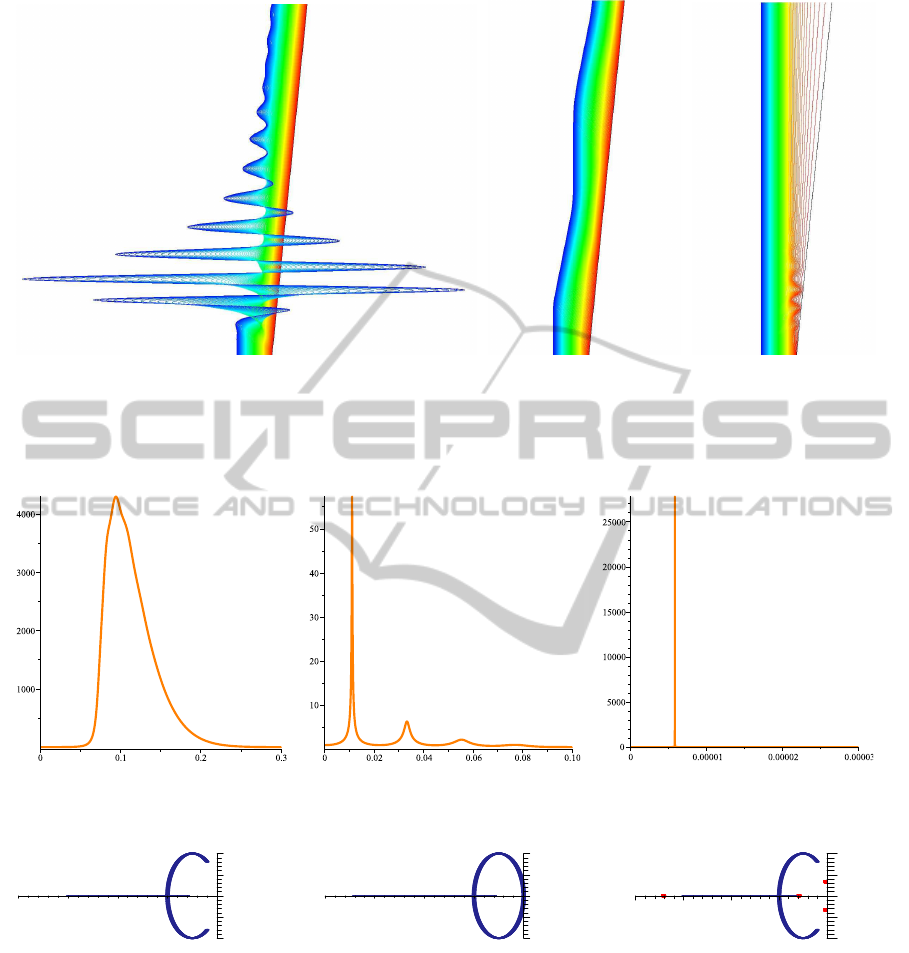
Figure 2: (color online) Numerical solution of the equation of motion of Definition 1.1 with r = ρ, f = −1, g = −2, N = 100.
Time (t) is vertical and position (x) is horizontal, each Figure being approximately a 1000 by 1000 square. Each agent initially
has unit distance to its neighbors, so that the flock initially is 100 units wide (horizontally). At t = 0 the rightmost agent, the
leader, starts moving with constant velocity 0.1 to the right. Simulations for ρ = 0.45 (left), ρ = 0.50 (middle), and ρ = 0.55
(right).
Figure 3: (color online) The frequency response function for the system of Figure 2. The absolute value of a
N
(ω) for ρ = 0.45
(left), ρ = 0.50 (middle), and ρ = 0.55 (right). Observe the different scales in these Figures!
−0.5
−3−4
0.0
−0.25
−2
0.25
0−1
0.5
−0.5
−3−4
0.0
−0.25
−2
0.25
0−1
0.5
0.25
−0.5
0−4 −1−2
−0.25
0.5
0.0
−3
Figure 4: (color online) Schematic representation in the complex plane of the eigenvalues associated to the first order ODE
of the system given in Figure 2. For ρ < 0.5 the real part of the eigenvalues are less than a negative constant (right). When ρ
approaches 0.5, the eigenvalues approximate the imaginary axis and the origin (middle). When ρ > 0.5 the process reverses,
except that two pairs of eigenvalues (in red) is spun off. One of these is exponentially (in N) close to zero (left).
independent of the topology of the network. We ex-
pect that similar equations can be written for flocks in
dimension 2 or 3.
5 CONCLUSIONS
The first point we argue in this position paper is
that considerations of a fundamental nature (symme-
try, friction) can help lead us to formulate the sim-
plest possible equations governing the motion of de-
PECCS 2011 - International Conference on Pervasive and Embedded Computing and Communication Systems
474

centralized flocks. In one dimension these are linear
(Proposition 2.1), but in higher dimension that is not
the case (Section 3). We contend that these equations
(especially the ones in dimension 2 or 3) have been
insufficiently studied in favor of ad hoc models. For
example it is not well-known enough that perturba-
tions cannot all die out as they travel through the flock
(Lemma 2.2. Neither do we know of any detailed
studies of flocks in R
2
or R
3
that change direction
and orientation s suggested in Section 3.
The second point we bring up is that of flock-
stability. In Definition 4.1 we propose that the stabil-
ity of a flock is determined by how certain response
functions grow with the size of the (homogeneous)
flock. A fundamental result, Theorem 4.2, states flock
stability is intimately related to internal symmetry of
the flock. This result together with Figure 4 shows
that it is completely misleading to look at the loca-
tion of the eigenvalues for these linear systems: one
must look at the time domain as well (the impulse re-
sponse function of Definition 4.1). This is not widely
acknowledged in the literature. Since time-domain re-
sults as those of Theorem 4.2) are so hard to obtain,
the need for new methods — preferably based on gen-
eral principles — is great. In Proposition 4.3 we pro-
pose to gain some insight in a general setting by eval-
uating the physical “work” done by the system.
ACKNOWLEDGEMENTS
I am grateful to Borko Stosic for numerous discus-
sions.
REFERENCES
Barooah, P. and Hespanha, J. P. (2005). Error amplification
and disturbance propagation in vehicle strings with
decentralized linear control. In IEEE conference on
decision and control, volume 5, pages 4964–4969.
Chandler, R. E., Herman, R., and Montroll, E. W. (1958).
Traffic dynamics: Studies in car following. Op. Res.,
6:165–184.
Chu, K.-C. (1974). Decentralized control of high-speed ve-
hicle strings. Transportation Science, 8(4):361–384.
DaFonseca, C. M. and Veerman, J. J. P. (2009). On the
spectra of certain directed paths. Appl. Math. Lett.,
9:1351–1355.
Herman, R., Montroll, E. W., Potts, R. B., and Rothery,
R. W. (1959). Traffic dynamics: Analysis and stability
in car following. Op. Res., 7:86–106.
Pant, A., Seiler, P., and Hedrick, K. (2002). Mesh stabil-
ity of look-ahead systems. IEEE Trans Aut. Contr.,
47(2):403–408.
Sullivan, W. (2010). Boundary Conditions and a One Lane
Linear model of Traffic Flow. Portland State Univer-
sity, Master’s Thesis.
Swaroop, D. and Hedrick, K. (1996a). String stability
of interconnected systems. IEEE Trans. Aut. Contr.,
41(3):349–357.
Swaroop, D. and Hedrick, K. (1996b). String stability
of interconnected systems. IEEE Trans. Aut. Contr.,
41(3):349–357.
Tangerman, F. M., Veerman, J. J. P., and Stosic, B. D.
(2010). Asymmetric decentralized flocks. Submitted.
Veerman, J. J. P. (2010). Stability of large flocks: an exam-
ple. arXiv:1002.0768.
Veerman, J. J. P., Caughman, J. S., Lafferriere, G., and
Williams, A. (2005). Flocks and formations. J. Stat.
Phys., 121(5-6):901–936.
Veerman, J. J. P., Stosic, B. D., and Tangerman, F. M.
(2009). Automated traffic and the finite size reso-
nance. J. Stat. Phys., 137(1):189–203.
Veerman, J. J. P. and Tangerman, F. M. (2010). Impulse sta-
bility of large flocks: an example. arXiv:1002.0782.
Williams, A., Lafferriere, G., and Veerman, J. (2005). Sta-
ble motions of vehicle formations. In IEEE 44th Conf.
on Decision and Contr., pages 72–77.
SYMMETRY AND STABILITY OF HOMOGENEOUS FLOCKS
475
