
STOCK MARKET FORECASTING BASED ON WAVELET AND
LEAST SQUARES SUPPORT VECTOR MACHINE
Xia Liang, Haoran Zhu and Xun Liang
School of Information, Renmin University of China, Beijing, China
Keywords: Wavelet transforms, Least squares support vector machine, Stock price prediction, Noisy signal, Machine
learning.
Abstract: In this paper, we propose a novel method using wavelet transform to denoise the input of least squares support
vector machine for classification of closing price of stocks. The proposed method classifies closing price as
either down or up. We have tested the proposed approach using passed three-year data of 10 stocks randomly
selected from sample stock of hs300 index and compared the proposed method with other machine learning
methods. Good classification percentage of almost 99% was achieved by WT-SVM model. We observed that
the performance of stock price prediction can be significantly enhanced by using hybrized WT in comparison
with a single model.
1 INTRODUCTION
Stock price prediction is an important financial
subject that has attracted lots of attentions from
researchers for many years(Liang et al,2009a). In the
past years, conventional statistical methods were
employed to forecast stock price. However, stock
price series are generally quite noisy and
non-stationary. To solve this problem, numerous
machine learning methods are adopted.
Tay and Cao(2001)used back-propagation neural
network and SVR and proved that SVR forecasts
better than BP neural network. Kim(2003)also used
BP and SVRs and in terms of movement direction it
proved that SVR outperformed back-propagation
neural network. Huang et al.
(2005) compared SVR
with linear discriminate analysis ,quadratic
discriminate analysis and Elman BPN and observed
that SVR forecasts better than other techniques in
terms of movement direction. Pai and Lin(2005)
proposed a hybrid model of ARIMA and SVM and
proved that the hybrid model forecasts better than
SVR and ARIMA.
Although SVM is useful in predicting the stock
price, lots of studies ignored the non-stationary of the
financial serials which are caused by political events,
economic conditions, traders’ expectations and other
environmental factors, are an important characteristic
of price serials(Abu&Atiya,1996). This variability
makes it difficult for any single machine learning
technique to capture the non-stationary property of
the data.
In our study, a prediction method using wavelet
transform to denoise the input of LS-SVM is
proposed. The performance between WT hybrid
model and single model are compared. All the models
are tested by past three-year financial serials of 10
stocks randomly selected from sample stocks of
hs300 index. The remainder of this paper are
organized as follows. In section 2, we introduce the
basic theory of WT and LS-SVM briefly. Section 3
gives the experiment scheme. The experiment results
are shown in Section 4. Finally conclusions are drawn
in Section 5.
2 THEORY OF WAVELET
TRANSFORM AND LS-SVM
2.1 Wavelet Transform
Wavelet is a kind of special waveform with limited
length and zero average (Chen&Guo,2005). Suppose
ψ
(t) is a quadratically integrable function, that is
ψ
(t) ∈ L
2
(R), if its Fourier transform satisfies the
following condition:
46
Liang X., Zhu H. and Liang X..
STOCK MARKET FORECASTING BASED ON WAVELET AND LEAST SQUARES SUPPORT VECTOR MACHINE.
DOI: 10.5220/0003436500460053
In Proceedings of the 13th International Conference on Enterprise Information Systems (ICEIS-2011), pages 46-53
ISBN: 978-989-8425-54-6
Copyright
c
2011 SCITEPRESS (Science and Technology Publications, Lda.)
=
|
(
)|
|
|
<+∞
(1)
Then
ψ
(t) is a basic wavelet or mother wavelet.
Equation (1) is the sufficient condition of mother
wavelet. By expanding and translating the wavelet
function, we can get
,
(
t
)
=
1
√
ψ
−
,>0,∈
(2)
a is called scale parameter and b is translation
parameter.
ψ
a,b
(t) is a wavelet function dependent on
parameter a and b. If a and b are continuous
parameters, then
ψ
a,b
(t) is a continuous wavelet
function. However, when using computer to deal with
signal, we usually use discrete wavelet function
instead and its reverse transform. Discrete wavelet
transform is as follows:
(
)
(
,
)
=
/
()Ψ
−
d (3)
is conjugate function of Ψ
.
The reverse of discrete wavelet:
(
)
=
〈
,
,
〉
∙
,
,
(
)
=
1
(
,
)
∙
,
,
(
)
(4)
In practice, useful signal is low frequency signal
or stationary signal while noise signal is high
frequency signal(Yin&Zheng,2004). To denoise the
signal, first we can use mother wavelet function to
decompose the signal and get the noise which is in the
high frequency component. Then we use threshold to
deal with the high frequency coefficients and we can
achieve the end by reconstructing all the components.
For the most popular denoising method, the signal is
firstly Fourier transformed and then using low-pass
filter among the frequency domain. As Fourier
transform cannot deal with time-frequency analysis,
it will smooth the mutations of the signal while
wavelet transform will keep mutations of the original
signal(Chen et al.,2001). So in order to denoise the
financial time serials, wavelet transform is a better
choice than Fourier transform. We can use wavelet
transform to denoise the signal by the below three
steps.
z Step 1 wavelet decomposition: choose the
wavelet and the decomposition level j and
then decompose the given signal. For
example if the decomposition level is three
the high frequency components will be
cD1-cD3 and low frequency will be cA3.
z Step 2 use threshold to denoise high
frequency coefficients: choose different
threshold value to modify the detail
coefficients for 1 to j-1 level.
z Steps 3 reconstruct the signal: based on the
low frequency coefficients and the modified
high frequency coefficients, reconstruct the
signal.
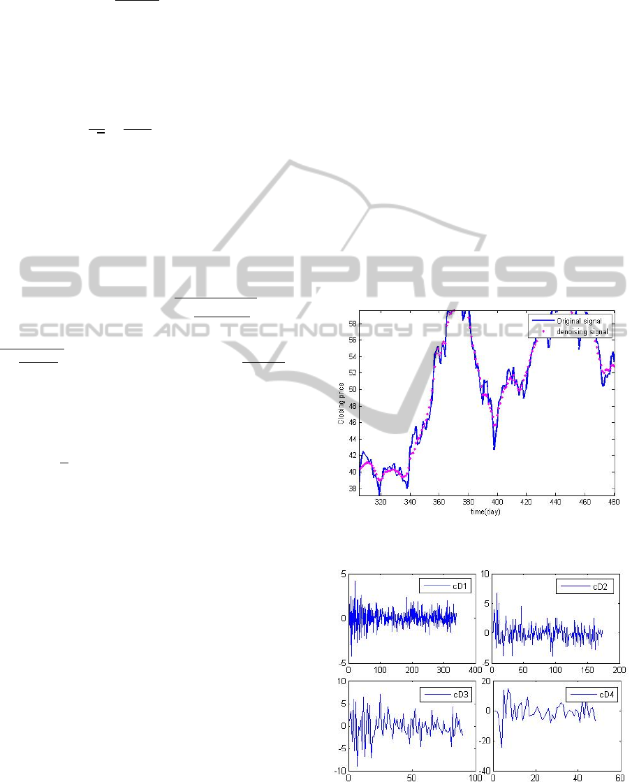
In Figure 1 the solid blue curve is the original
financial signal and the dashed red one is
reconstructed with WT. We can see that the denoised
signal is much smoother and less fluctuate than the
original one. Figure 2 shows its four components in
details, cD1-cD4, obtained after the application of the
WT. These details correspond to the highest
frequency components of the signal using different
sizes of time windows for each scales(Mallat,1999).
Figure 1: The original signal (blue solid curve) and
denoised signal obtained with WT (red dot).
Figure 2: Signal’s components of details cD1-cD4 obtained
with WT.
STOCK MARKET FORECASTING BASED ON WAVELET AND LEAST SQUARES SUPPORT VECTOR MACHINE
47

2.2 The Least Squares Support Vector
Machine (LS-SVM)
The standard SVM is solved by using quadratic
programming methods. However, these methods are
often time consuming and are difficult to implement
adaptively. Least squares support vector machines
(LS-SVM) is capable of solving both classification
and regression problems and is receiving more and
more attention, because it has some properties related
to the implementation and computational method
(Suykens&Vandewalle, 1999; Suykens et al., 2002).
For example, training requires solving a set of linear
equations instead of solving the quadratic
programming problem involved in the original SVM,
and consequently the global minizer is much easier to
obtain. The original SVM formulation of Vapnik
(1998) is modified by considering equality
constraints within a form of ridge regression rather
than considering inequality constraints. In LS-SVM,
the Vapnik’s standard SVM classifier was modified
into the following formulation(Zheng et al.,2004):
2
1
11
min ( (5)
22
n
T
k
k
J ω,b,ξ)= ωω+ γ e
=
∑
Subjected to
[ ( ) ] 1 1,....,
T
ii k
y ωτ
x
beandk n+=− =
The corresponding Lagrange for Equation (5) is
()()
()
[]
{}
1
,,, , ,
1,(6)
n
T
kk k k
k
Lbe J be
yxbe
ωα ω
αωτ
=
=
−+−+
∑
α
k
is the Lagrange multiplier shown in
Ref(
Cristianini&Shawe,2000).The optimality
condition leads to the following [(N+1)× [N+1]]
linear system:
1
0
0Y
(7)
1
Y
T
T
b
ZZ I
α
γ
−
⎛⎞
⎛⎞⎛⎞
=
⎜⎟
⎜⎟⎜⎟
+
⎝⎠⎝⎠
⎝⎠
Where
1
11
1
() ,...,()
[ ,..., ]; [ ,..., ] (8)
i
i
nn
T
y
T
Zxy x
Yy y and
ττ
αα α
⎡⎤
=
⎢⎥
⎣⎦
==
In this paper LS-SVR represents least squares
support machine regression and LS-SVC represents
support machine classification.
3 EXPERIMENT DESIGN
3.1 Data Collection
We obtain the recent three year data from the finance
section of Yahoo. The whole data set covers the
period from January 1, 2008 to Dec 31, 2010 of 10
stocks. Each daily observation includes 6 indicators:
opening price, highest price, lowest price, closing
price, volume, and turnover. We examined 10
random stocks whose code can be found in Table 5.
We believe that the time periods cover many
important economic events, which are sufficient for
testing the issue of non-stationary properties inherent
in financial data.
3.2 Model Inputs & Outputs Design
For machine learning techniques combining with
WT, Original closing price was first decomposed and
reconstructed using wavelet transform. Symbol data
2008_2010 represents the original data and XC is
obtained from the closing price processed by WT. We
tried to design the input variables. Input variables
include VolumeIndex, CloseIndex, MeanClose,
RangeIndex, MaxHigh, MinLow, TurnoverIndex. All
of them were transformed according to passed 10-day
data. This design may improve the predictive power
of artificial methods. The output variable is
L+1-close. The input variables are determined by
lagged data2008_2010 values based on L-day
periods. L is the time window which is set to 10.In our
study we predict the closing price of 11
th
day based
on the last 10-day information. The calculations for
all variables can be found in Table 1. All the values
were first scaled into the range of [-1, 1] to normalize
each feature component so that larger input attributes
do not overwhelm smaller inputs. 500 observations
were used for training and 100 for testing.
3.3 Performance Criteria
The prediction performance is evaluated using the
following statistical methods: mean absolute
percentage error (MAPE), directional symmetry (DS)
and weighted directional symmetry
(WDS)(Kim,2003). The definitions of these criteria
can be found in Table 2.MAPE is the measure of the
deviation between actual values and predicted values.
The smaller the values of MAPE, the closer are the
predicted time series values in relation to the actual
values. Although predicting the actual levels of price
changes is desirable, in many cases, the direction of
the
change is equally important. DS provides the
ICEIS 2011 - 13th International Conference on Enterprise Information Systems
48

Table 1: Input and output variables.
Feature Calculation
Input variable
VolumeIndex data2008_2010 (L+i-1,6)/mean(data2008_2010 (i:L-1+i,6))
CloseIndex data2008_2010 (L+i-1,5)/mean(data2008_2010 (i:L-1+i,5))
MeanClose Noise:Mean(data2008_2010 (i:L-1+i,5)) Denoise:Mean(XC(i:L-1+i,5))
RangeIndex max(data2008_2010(i:L-1+i,3))-min(data2008_2010(i:L-1+i,4))
MaxHigh max(data2008_2010(i:L-1+i,3))
MinLow min(data2008_2010(i:L-1+i,4))
TurnoverIndex mean(data2008_2010(i:L-1+i,7))
Output variable
L+1-Close Noise:data2008_2010(L+i,5)
1
,signfdata2008_2010(L+i,5)-data2008_2010(L+i-1,5))
2
;Denoise:
XC(L+i,1)
1
, signf(XC(L+i,1)-XC(L+i-1,1))
2
Notes:1 –while using LS-SVR;2-while using LS-SVC;signf
(
x
)
=
−1, x<0
1, x≥0
Table 2: Performance criteria and their calculation.
Metric Calculation
MAPE MAPE=(1/n)*∑
i=1
n
|a
i
-p
i
|
DS DS=1/n*∑
i=1
n
d
i
d
=
1
(
a
−p
)(
p
−p
)
0
WDS WDS=∑
i=1
n
d
i
*|a
i
-p
i
|/∑
i=1
n
d
i
’*|a
i
-p
i
|
d
=
0
(
a
−p
)(
p
−p
)
1
d
=
1
(
a
−p
)(
p
−p
)
0
correctness of the predicted direction of closing price
in terms of percentage; the larger values of DS
suggest a better predictor. WDS measures the
magnitude of the prediction error as well as the
direction. It penalizes error related to incorrectly
predicted directions and rewards those associated
with correctly predicted directions. The smaller the
value of WDS, the better is the forecasting
performance in terms of both magnitude and
direction.
3.4 Wavelet Denoising Implementation
There are two metrics to evaluate the performance of
WT denoisng. One is PERFL2 (Accardo&Mumolo,
1998).It is a percentage, representing how much
energy and mutations are reserved from the original
signal. The larger PERFL2 , the better wavelet
denoising will be. The other is norm of the difference
between original signal and reconstructed signal. The
smaller the norm, the more approximate the
reconstructed signal will be to the original signal.
For the process of WT denoising implementation,
there are two significant things-determining the
wavelet function and the threshold function. As the
wavelet function is not unique, different wavelet
functions may lead to absolutely different results.
Thus, it is a key point to choose an appropriate
wavelet function. Below we used the same threshold
which is automatically got by the ‘minimaxi’
function(FeiSi,2005) and compared three main
wavelet functions’ denoising effect. From Table 3 we
can see that wavelet function ‘sym6’ gives the best
STOCK MARKET FORECASTING BASED ON WAVELET AND LEAST SQUARES SUPPORT VECTOR MACHINE
49
denoising effect. The PERFL2 of ‘sym6’ is the
largest which means it removes the noise and keeps
the mutations of the original signal best. The Norm of
‘sym6’ is the smallest, that is to say, the reconstructed
signal is most appropriate to the original signal. Table
4 demonstrates that the threshold function ‘minmaxi’
is the best choice whose PERFL2 is the largest and
the Norm is the smallest.
Table 3: Denoising effect of different wavelet.
Wavelet function PERFL2 Norm
sym6 99.9366 25.7364
db4 99.9305 26.4097
Haar 99.9305 26.4097
Table 4: Denoisng effect of different threshold.
threshold rules PERFL2 Norm
Minmaxi 99.9366 25.7364
Rigrsure 99.9143 35.1875
Heursure 99.9291 26.6613
3.5 LS-SVM Prediction
Implementation
The typical kernel functions are the polynomial
kernel k(x,y)=(x*y+1)
d
and the RBF kernel
k(x,y)=exp(-(x-y)
2
/σ
2
), where d is the degree of the
polynomial kernel and σ
2
is the bandwidth of the RBF
kernel(
Goudarzi&Goodarzi,2008). In our
experiment, we chose the RBF kernel as our kernel
function because it tends to achieve better
performance (Liang&Wang, 2009b). The specific
steps are as follows:
z Step 1: Define N as the size of training data and
M as the size of testing data. Choose N+M
random unrepeated data from the normalized
data set. The former N will be used to training
the SVM model and the latter M will be used to
test the model performance. In our experiment
we set N=500, M=100.
z Step2: Train the SVR and SVC model by
choosing the LS-SVM type as ‘function
estimation’ and ‘classification’ respectively.
z Step3: Compute the metrics.
z Step4: Repeat all the steps for 10 selected
stocks.
3.6 Other Machine Learning Methods
In order to prove the better performance of wavelet
transform denoisng and the high prediction of
LS-SVM, we chose two neural network methods to
predict the financial signal and compare their
performance(Gao,2007).
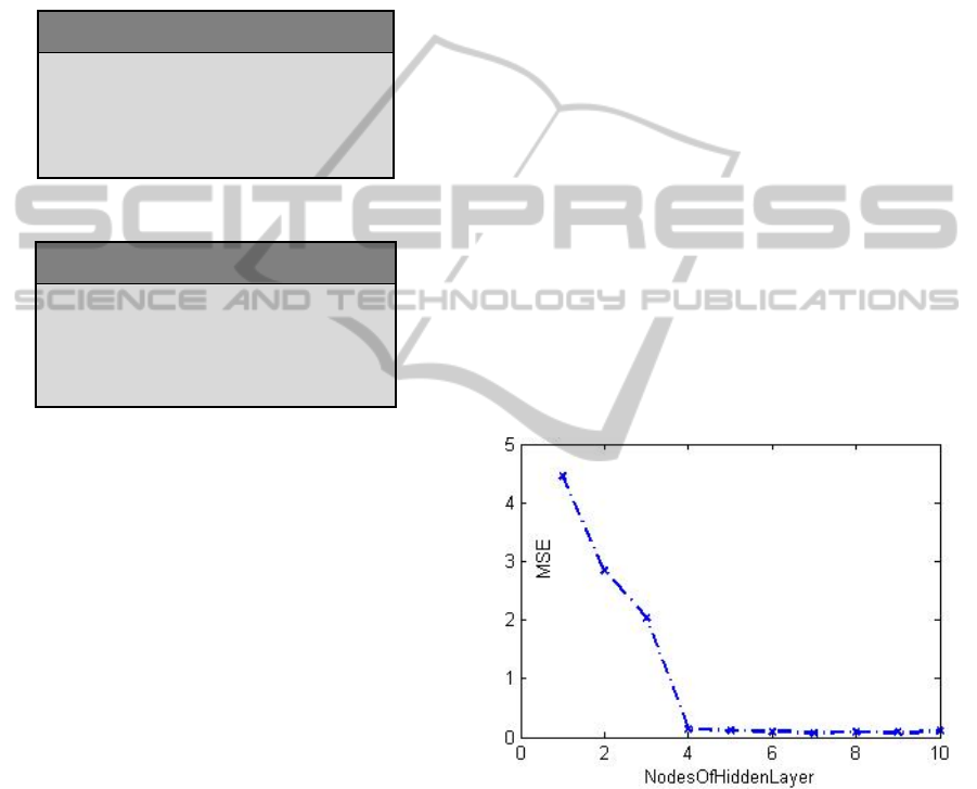
First, we established the BP neural network model
using the data defined by Table 1.The difficulty in
building the BP model is to find the best number of
nodes of the hidden layer (which we define as m).
According to formulation m = sqrt (n+l) +a (n is the
number of the nodes of input Layer and l is number of
nodes of output Layer), we get Figure 3 which prove
that when m equals eight, the model will perform
very well.
Second, we used the same time serials to build a
RBF (radius bias function) neural network
model.RBF neural network is a kind of efficient
feed-forward neural network, having best
approximation property and global optimal
performance which other networks do not have. Its
structure is very simple and the model training is very
fast. Meanwhile, the RBF neural network is also
widely used in pattern recognition, nonlinear pattern
recognition and the field of nonlinear neural network
modelling.
Figure 3: Nodes of hidden layer of BPN.
4 EXPERIMENT RESULTS
The results of single LS-SVM and WT-LS-SVM
model are shown in Table 5. The values of DS are
larger in the SVRs than in the SVCs and larger in the
WT model than the single model. This suggests that
in terms of correctness of the predicted direction of
closing price, the SVRs and WT model offers better
prediction and WT-SVRs give the best prediction.
ICEIS 2011 - 13th International Conference on Enterprise Information Systems
50

The results are tested and consistent in all 10 stock
data sets. Figure 4 shows that the WT hybrid model
outperforms the single SVM model.
In Figure 4, for the x axis, the Ci(i=1,2,…,10)
points are the values of SVCs and the Ri(i=1,2,…,10)
points are the results of SVRs. Table 5 and Figure 4
demonstrate that when the data is denoised by
wavelet transformation the prediction result is more
accurate and the deviation between the actual value
and prediction value is smaller. Specifically,
(1) SVRs has a accuracy rate more than 90% in
both single SVM and WT-SVM model. That means
SVR has a good ability to deal with outliers.
(2) The performance of SVCs is improved greatly
from less 50% to more than 80% after hybrid with
WT.
To better prove the effectiveness of wavelet
transform, we compared the performance of SVM
with that of BP and RBF neural network. The fitting
comparisons are shown in Figure 5 and the prediction
performance is shown in Table 6.
From Figure 5 we can see that the fitting values of
all the methods except BP are extremely approximate
to the original values. For BP, the hybrid model
outperforms greatly than the single BP.
Figure 4: DS of single SVM and WT-SVM.
The results of different machine learning methods
are shown in Table 6. In terms of MAPE, WDS,
we
observe that the WT hybrid model achieves
smaller values than the single model does on the
testing data set. This suggests that the WT model can
have smaller deviations between predicted values and
actual ones than the single model. The values of DS
are
larger in the WT model than single model. This
Table 5: Prediction performance of single SVM and WT model.
StockCode DS WT-DS StockCode DS WT-DS
601328 0.476(SVC) 0.855(SVC) 600102 0.501(SVC) 0.804(SVC)
0.966(SVR) 0.99(SVR) 0.965(SVR) 0.998(SVR)
600016 0.479(SVC) 0.866(SVC) 600282 0.488(SVC) 0.855(SVC)
0.971(SVR) 0.996(SVR) 0.986(SVR) 0.996(SVR)
601166 0.501(SVC) 0.781(SVC) 601003 0.472(SVC) 0.857(SVC)
0.966(SVR) 0.991(SVR) 0.962(SVR) 0.995(SVR)
600036 0.482(SVC) 0.855(SVC) 600376 0.509(SVC) 0.854(SVC)
0.965(SVR) 0.997(SVR) 0.975(SVR) 0.975(SVR)
601318 0.517(SVC) 0.719(SVC) 600350 0.505(SVC) 0.854(SVC)
0.971(SVR) 0.989(SVR) 0.948(SVR) 0.993(SVR)
Table 6: Prediction performance of different methods.
SVM
WT
SVM
BP
WT
BP
RBF
WT
RBF
MAPE 1.33 1.25 9.29 6.45 1.43 1.27
DS 0.97 0.99 0.87 0.91 0.96 0.97
WDS 0.03 0 0.16 0.1 0.05 0.03
STOCK MARKET FORECASTING BASED ON WAVELET AND LEAST SQUARES SUPPORT VECTOR MACHINE
51
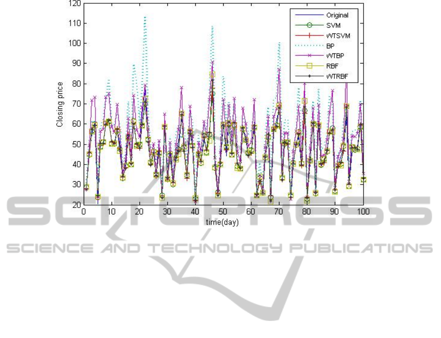
Figure 5: Fitting values of different methods.
suggests that in terms of correctness of the predicted
direction of closing price, the WT model gives better
prediction. Comparing WT-RBF with SVM, we can
see that the values of their DS and WDS are the same
while the MAPE of WT-RBF is smaller than that of
single SVM.That means the WT-RBF model can
have smaller deviations between predicted values and
actual ones than the single SVM model. Thus, the
SVR model does not outperform the neural network
model which is not consistent with the conclusions of
most of recent studies like Huang et al. (2005).
5 CONCLUSIONS AND FUTURE
WORK
This study used LS-SVM to predict future direction
of stock price and the effect of the noise of time
serials in LS-SVM was considered. The experiment
results showed that the prediction performance was
increased by using wavelet transform hybrid model.
In addition, this study compared SVM model with
other machine learning methods. The experiment
results showed that single SVM may not have better
prediction performance than RBF neural network
model which is different from general studies. Hybrid
with wavelet transform, SVR model becomes
absolutely perfect as in terms of correctness of the
predicted direction of closing price. In this paper we
can see the WT-SVM model always gives above 90%
accuracy.
There are some other issues which may enhance
the prediction performance of SVM. For instance, the
sentiment analysis of financial news will be a very
interesting topic in the future. Whether the sentiment
value is a kind of noise needs to further study. The
feature vector based on wavelet transform mentioned
above has a good performance, but this vector might
not be the optimal choice. Therefore, the research on
the comparison of feature vector adding the sentiment
value is our following work.
ACKNOWLEDGEMENTS
This work was supported by the Fundamental
Research Funds for the Central Universities, and the
Research Funds of Renmin University of China plus
10XNI029 plus Research on Financial Web Data
Mining and Knowledge Management, the Natural
Science Foundation of China under grant 70871001,
and the 863 Project of China under grant
2007AA01Z437.
REFERENCES
Abu-Mostafa, Y. S., & Atiya, A. F., 1996. Introduction to
financial forecasting. Applied Intelligence, 6(3),
205-213.
Accardo, A. P., & Mumolo, E.,1998. An algorithm for the
automatic differentiation between the speech of
ICEIS 2011 - 13th International Conference on Enterprise Information Systems
52

normals and patients with Friedreich’s ataxia based on
the short-time fractal dimension. Computers in Biology
and Medicine, 28(1), 75-89.
Available from http://www.mathworks.com.[Accessed on
20th Jan, 2011].
Chen, G. M., Zhang, M. Z., & Qi, Y. H., 2001. Application
of MATLAB language processing digital signals and
digital image. Beijing: Science Press, 125-127.
Chen, L. Z., & Guo, H, W., 2005. Discrete wavelet
transform theory and engineering practice. Beijing:
Tsinghua University Press, 9-15.
Cristianini, N., Shawe-Taylor, J., 2000. An Introduction to
Support Vector Machines and Other Kernel-based
Learning Methods. Cambridge:Cambridge University
Press.
FeiSi Technology R & D centre 2005. Wavelet analysis
theory and the implementation with MATLAB7. Beijing:
Electronic Industry Press, 328-330.
Gao, Q., 2007. The application of artificial nerve network
in the stock market forecast model. Microeclctronics&
Computer, 24(11), 147-151.
Goudarzi, N., & Goodarzi, M., 2008. Prediction of the
logarithmic of partition Nasser, etc. coefficients(log P)
of some organic compounds by least square-support
vector machine(LS-SVM). Molecular Physics,
106(21-23), 2525-2535.
Huang, W., Nakamori, Y., & Wang, S. Y., 2005.
Forecasting stock market movement direction with
support vector machine. Computers & Operations
Research, 32(10), 2513-2522.
Kim, K. J., 2003. Financial time series forecasting using
support vector machines. Neurocomputing, 55(1-2),
307-319.
Liang, X., Zhang, H. S., Xiao, J. G., & Chen, Y., 2009a.
Improving option price forecasts with neural networks
and support vector regressions. Neurocomputing,
72(13-15), 3055-3065.
Liang, X., & Wang, C., 2009b. Separating hypersurfaces of
SVMs in input spaces. Pattern Recognition Letters,
30(5), 469-476.
Mallat, S. G., 1999. A Wavelet Tour of Signal Processing.
San Diego: Academic Press.
Pai, P.-F., & Lin, C.-S. (2005). A hybrid ARIMA and
support vector machines model instock price
forecasting. Omega, 33, 497–505.
Strang, G., & Nguyen, T., 1997. Wavelets and Filter Banks.
Wellesley: Wellesley-Gambridge Academic Press.
Suykens, J. A. K., & Vandewalle, J., 1999. Least squares
support vector machine classifiers. Neural processing
letters, 9(3), 293-300.
Suykens, J. A. K., Gestel, T. V., Brabanter, J. D., Moor, B.
D., &Vandewalle, J., 2002. Least Squares Support
Vetor Machine Classifiers. Singapore: World Scientific
Publishing Co. Pte.Ltd.
Tay, F.E.H., &Cao, L.J., 2001. Application of support
vector machines in financial time series forecasting.
Omega, 29, 309-317
Vapnik, V. N., 1998. Statistical Learning Theory, Wiley,
New York.
Yin, G. W., & Zheng, P. E., 2004. Forecasting stock market
using wavelet theory. Systems engineering-theory
methodology applications, 13(6), 543-547.
Zheng, S., Liu, L., & Tian, J. W., 2004. A new efficient
SVM-based edge detection method. Pattern
Recognition Letters, 25(10), 1143-1154.
STOCK MARKET FORECASTING BASED ON WAVELET AND LEAST SQUARES SUPPORT VECTOR MACHINE
53
