RANDOM BUILDING BLOCK OPERATOR FOR GENETIC

ALGORITHMS

Ghodrat Moghadampour

VAMK, University of Applied Sciences, Technology and Communication, Wolffintie 30, 65200, Vaasa, Finland

Keywords: Evolutionary algorithm, Genetic algorithm, Function optimization, Mutation operator, Multipoint mutation

operator, Random building block operator, Fitness evaluation and analysis.

Abstract: Genetic algorithms work on randomly generated populations, which are refined toward the desired optima.

The refinement process is carried out mainly by genetic operators. Most typical genetic operators are

crossover and mutation. However, experience has proved that these operators in their classical form are not

capable of refining the population efficiently enough. Moreover, due to lack of sufficient variation in the

opulation, the genetic algorithm might stagnate at local optimum points. In this work a new dynamic

mutation operator with variable mutation rate is proposed. This operator does not require any pre-fixe

parameter. It dynamically takes into account the size (number of bits) of the individual during runtime an

replaces a randomly selected section of the individual by a randomly generated bit string of the same size.

All the bits of the randomly generated string are not necessarily different from bits of the selected section

from the individual. Experimentation with 17 test functions, 34 test cases and 1020 test runs proved the

superiority of the proposed dynamic mutation operator over single-point mutation operator with 1%, 5% an

8% mutation rates and the multipoint mutation operator with 5%, 8% and 15% mutation rates.

1 INTRODUCTION

Evolutionary algorithms are heuristic algorithms,

which imitate the natural evolutionary process and

try to build better solutions by gradually improving

present solution candidates. It is generally accepted

that any evolutionary algorithm must have five basic

components: 1) a genetic representation of a number

of solutions to the problem, 2) a way to create an

initial population of solutions, 3) an evaluation

function for rating solutions in terms of their

“fitness”, 4) “genetic” operators that alter the genetic

composition of offspring during reproduction, 5)

values for the parameters, e.g. population size,

probabilities of applying genetic operators

(Michalewicz, 1996).

A genetic algorithm is an evolutionary algorithm,

which starts the solution process by randomly

generating the initial population and then refining

the present solutions through natural like operators,

like crossover and mutation. The behaviour of the

genetic algorithm can be adjusted by parameters,

like the size of the initial population, the number of

times genetic operators are applied and how these

genetic operators are implemented. Deciding on the

best possible parameter values over the genetic run

is a challenging task, which has made researchers

busy with developing even better and efficient

techniques than the existing ones.

2 GENETIC ALGORITHM

Most often genetic algorithms (GAs) have at least

the following elements in common: populations of

chromosomes, selection according to fitness,

crossover to produce new offspring, and random

mutation of new offspring.

A simple GA works as follows: 1) A population of

-bit strings (chromosomes) is randomly

generated, 2) the fitness

)(xf of each chromosome

in the population is calculated, 3) chromosomes

are selected to go through crossover and mutation

operators with

p and

p probabilities respectively,

4) the old population is replaced by the new one, 5)

the process is continued until the termination

conditions are met.

However, more sophisticated genetic algorithms

typically include other intelligent operators, which

Moghadampour G..

RANDOM BUILDING BLOCK OPERATOR FOR GENETIC ALGORITHMS.

DOI: 10.5220/0003441400540062

In Proceedings of the 13th International Conference on Enterprise Information Systems (ICEIS-2011), pages 54-62

ISBN: 978-989-8425-54-6

 2011 SCITEPRESS (Science and Technology Publications, Lda.)

apply to the specific problem. In addition, the whole

algorithm is normally implemented in a novel way

with user-defined features while for instance

measuring and controlling parameters, which affect

the behaviour of the algorithm.

2.1 Genetic Operators

For any evolutionary computation technique, the

representation of an individual in the population and

the set of operators used to alter its genetic code

constitute probably the two most important

components of the system. Therefore, an appropriate

representation (encoding) of problem variables must

be chosen along with the appropriate evolutionary

computation operators. The reverse is also true;

operators must match the representation. Data might

be represented in different formats: binary strings,

real-valued vectors, permutations, finite-state

machines, parse trees and so on. Decision on what

genetic operators to use greatly depends on the

encoding strategy of the GA. For each

representation, several operators might be employed

(Michalewicz, 2000). The most commonly used

genetic operators are crossover and mutation. These

operators are implemented in different ways for

binary and real-valued representations. In the

following, these operators are described in more

details.

2.1.1 Crossover

Crossover is the main distinguishing feature of a

GA. The simplest form of crossover is single-point:

a single crossover position is chosen randomly and

the parts of the two parents after the crossover

position are exchanged to form two new individuals

(offspring). The idea is to recombine building blocks

(schemas) on different strings. However, single-

point crossover has some shortcomings. For

instance, segments exchanged in the single-point

crossover always contain the endpoints of the

strings; it treats endpoints preferentially, and cannot

combine all possible schemas. For example, it

cannot combine instances of 11*****1 and

****11** to form an instance of 11***11*(Mitchell,

1998). Moreover, the single-point crossover suffers

from “positional bias” (Mitchell, 1998): the location

of the bits in the chromosome determines the

schemas that can be created or destroyed by

crossover.

Consequently, schemas with long defining lengths

are likely to be destroyed under single-point

crossover. The assumption in single-point crossover

is that short, low-order schemas are the functional

building blocks of strings, but the problem is that the

optimal ordering of bits is not known in advance

(Mitchell, 1998). Moreover, there may not be any

way to put all functionally related bits close together

on a string, since some particular bits might be

crucial in more than one schema. This might happen

if for instance in one schema the bit value of a locus

is 0 and in the other schema the bit value of the same

locus is 1. Furthermore, the tendency of single-point

crossover to keep short schemas intact can lead to

the preservation of so-called hitchhiker bits. These

are bits that are not part of a desired schema, but by

being close on the string, hitchhike along with the

reproduced beneficial schema (Mitchell, 1998).

In two-point crossover, two positions are chosen at

random and the segments between them are

exchanged. Two-point crossover reduces positional

bias and endpoint effect, it is less likely to disrupt

schemas with large defining lengths, and it can

combine more schemas than single-point crossover

(Mitchell, 1998). Two-point crossover has also its

own shortcomings; it cannot combine all schemas.

Multipoint-crossover has also been implemented,

e.g. in one method, the number of crossover points

for each parent is chosen from a Poisson distribution

whose mean is a function of the length of the

chromosome. Another method of implementing

multipoint-crossover is the “parameterized uniform

crossover” in which each bit is exchanged with

probability

, typically 8.05.0 ≤≤ p (Mitchell,

1998). In parameterized uniform crossover, any

schemas contained at different positions in the

parents can potentially be recombined in the

offspring; there is no positional bias. This implies

that uniform crossover can be highly disruptive of

any schema and may prevent coadapted alleles from

ever forming in the population (Mitchell, 1998).

There has been some successful experimentation

with a crossover method, which adapts the

distribution of its crossover points by the same

process of survival of the fittest and recombination

(Michalewicz, 1996). This was done by inserting

into the string representation special marks, which

keep track of the sites in the string where crossover

occurred. The hope was that if a particular site

produces poor offspring, the site dies off and vice

versa.

The one-point and uniform crossover methods

have been combined by some researchers through

extending a chromosomal representation by an

additional bit. There has also been some

experimentation with other crossovers: segmented

crossover and shuffle crossover (Eshelman et al.,

RANDOM BUILDING BLOCK OPERATOR FOR GENETIC ALGORITHMS

1991; Michalewicz, 1996). Segmented crossover, a

variant of the multipoint, allows the number of

crossover points to vary. The fixed number of

crossover points and segments (obtained after

dividing a chromosome into pieces on crossover

points) are replaced by a segment switch rate, which

specifies the probability that a segment will end at

any point in the string. The shuffle crossover is an

auxiliary mechanism, which is independent of the

number of the crossover points. It 1) randomly

shuffles the bit positions of the two strings in

tandem, 2) exchanges segments between crossover

points, and 3) unshuffles the string (Michalewicz,

1996). In gene pool recombination, genes are

randomly picked from the gene pool defined by the

selected parents.

There is no definite guidance on when to use

which variant of crossover. The success or failure of

a particular crossover operator depends on the

particular fitness function, encoding, and other

details of GA. Actually, it is a very important open

problem to fully understand interactions between

particular fitness function, encoding, crossover and

other details of a GA. Commonly, either two-point

crossover or parameterized uniform crossover has

been used with the probability of occurrence

8.07.0 −≈p (Mitchell, 1998).

Generally, it is assumed that crossover is able to

recombine highly fit schemas. However, there is

even some doubt on the usefulness of crossover, e.g.

in schema analysis of GA, crossover might be

considered as a “macro-mutation” operator that

simply allows for large jumps in the search space

(Mitchell, 1998).

2.1.2 Mutation

The common mutation operator used in canonical

genetic algorithms to manipulate binary strings

}1,0{),...(

=∈= Iaaa of fixed length A was

originally introduced by Holland (Holland, 1975) for

general finite individual spaces

AAI ...

×= , where

},...,{

iii

= . By this definition, the mutation

operator proceeds by:

i. determining the position

}),...,1{(,...,

liii

∈ to

undergo mutation by a uniform random

choice, where each position has the same

small probability

p of undergoing mutation,

independently of what happens at other

position

ii. forming the new vector

),...,,,...,,,,...,(

1 A

aaa

hhh

+−

′

where

∈

′

is drawn uniformly at random

from the set of admissible values at position

i .

The original value

a at a position undergoing

mutation is not excluded from the random choice of

Aa ∈

′

. This implies that although the position is

chosen for mutation, the corresponding value might

not change at all (Bäck et al., 2000).

Mutation rate is usually very small, like 0.001

(Mitchell, 1998). A good starting point for the bit-

flip mutation operation in binary encoding is

, where L is the length of the chromosome

(Mühlenbein, 1992). Since

corresponds to

flipping one bit per genome on average, it is used as

a lower bound for mutation rate. A mutation rate of

range

[

]

01.0,005.0∈

P is recommended for binary

encoding (Ursem, 2003). For real-value encoding

the mutation rate is usually

[]

9.0,6.0∈

P and the

crossover rate is

[

]

0.1,7.0∈

(Ursem, 2003).

Crossover is commonly viewed as the major

instrument of variation and innovation in GAs, with

mutation, playing a background role, insuring the

population against permanent fixation at any

particular locus (Mitchell, 1998; Bäck et al., 2000).

Mutation and crossover have the same ability for

“disruption” of existing schemas, but crossover is a

more robust constructor of new schemas (Spears,

1993; Mitchell, 1998). The power of mutation is

claimed to be underestimated in traditional GA,

since experimentation has shown that in many cases

a hill-climbing strategy works better than a GA with

crossover (Mühlenbein, 1992; Mitchell, 1998).

While recombination involves more than one

parent, mutation generally refers to the creation of a

new solution from one and only one parent. Given a

real-valued representation where each element in a

population is an

n -dimensional vector

ℜ∈ , there

are many methods for creating new offspring using

mutation. The general form of mutation can be

written as:

)(xmx

′

(1)

where

is the parent vector, m is the mutation

function and

′

is the resulting offspring vector. The

more common form of mutation generated offspring

vector:

ICEIS 2011 - 13th International Conference on Enterprise Information Systems

Mxx +=

′

(2)

where the mutation

M is a random variable. M has

often zero mean such that

xxE =

′

)(

(3)

the expected difference between the real values of a

parent and its offspring is zero (Bäck et al., 2000).

Some forms of evolutionary algorithms apply

mutation operators to a population of strings without

using recombination, while other algorithms may

combine the use of mutation with recombination.

Any form of mutation applied to a permutation must

yield a string, which also presents a permutation.

Most mutation operators for permutations are related

to operators, which have also been used in

neighbourhood local search strategies (Whitley,

2000). Some other variations of the mutation

operator for more specific problems have been

introduced in (Bäck et al., 2000). Some new

methods and techniques for applying crossover and

mutation operators have also been presented in

(Moghadampour, 2006).

It is not a choice between crossover and mutation

but rather the balance among crossover, mutation,

selection, details of fitness function and the

encoding. Moreover, the relative usefulness of

crossover and mutation change over the course of a

run. However, all these remain to be elucidated

precisely (Mitchell, 1998).

2.1.3 Other Operators and Mating

Strategies

In addition to common crossover and mutation there

are some other operators used in GAs including

inversion, gene doubling and several operators for

preserving diversity in the population. For instance,

a “crowding” operator has been used in (De Jong,

1975; Mitchell, 1998) to prevent too many similar

individuals (“crowds”) from being in the population

at the same time. This operator replaces an existing

individual by a newly formed and most similar

offspring. In (Mengshoel et al., 2008) a probabilistic

crowding niching algorithm in which subpopulations

are maintained reliably, is presented. It is argued that

like the closely related deterministic crowding

approach, probabilistic crowding is fast, simple, and

requires no parameters beyond those of classical

genetic algorithms.

The same result can be accomplished by using an

explicit “fitness sharing” function (Mitchell, 1998),

whose idea is to decrease each individual’s fitness

by an explicit increasing function of the presence of

other similar population members. In some cases,

this operator induces appropriate “speciation”,

allowing the population members to converge on

several peaks in the fitness landscape (Mitchell,

1998). However, the same effect could be obtained

without the presence of an explicit sharing function

(Smith et al., 1993; Mitchell, 1998).

Diversity in the population can also be promoted

by putting restrictions on mating. For instance,

distinct “species” tend to be formed if only

sufficiently similar individuals are allowed to mate

(Mitchell, 1998). Another attempt to keep the entire

population as diverse as possible is disallowing

mating between too similar individuals, “incest”

(Eshelman et al., 1991; Mitchell, 1998). Another

solution is to use a “sexual selection” procedure;

allowing mating only between individuals having

the same “mating tags” (parts of the chromosome

that identify prospective mates to one another).

These tags, in principle, would also evolve to

implement appropriate restrictions on new

prospective mates (Holland, 1975).

Another solution is to restrict mating spatially.

The population evolves on a spatial lattice, and

individuals are likely to mate only with individuals

in their spatial neighborhoods. Such a scheme would

help preserve diversity by maintaining spatially

isolated species, with innovations largely occurring

at the boundaries between species (Mitchell, 1998).

The efficiency of genetic algorithms has also

been tried by imposing adaptively, where the

algorithm operators are controlled dynamically

during runtime (Eiben et al. 2008). These methods

can be categorized as deterministic, adaptive, and

self-adaptive methods (Eiben & Smitt, 2007; Eiben

et al. 2008). Adaptive methods adjust the

parameters’ values during runtime based on

feedback from the algorithm (Eiben et al. 2008),

which are mostly based on the quality of the

solutions or speed of the algorithm (Smit et al.,

2009).

3 THE RANDOM BUILDING

BLOCK OPERATOR

The random building block (RBB) operator is a new

self-adaptive operator proposed here. During the

classical crossover operation, building blocks of two

or more individuals of the population are exchanged

in the hope that a better building block from one

individual will replace a worse building block in the

other individual and improve the individual’s fitness

value. However, the random building block operator

involves only one individual. The random building

RANDOM BUILDING BLOCK OPERATOR FOR GENETIC ALGORITHMS

block operator resembles more the multipoint

mutation operator, but it lacks the frustrating

complexity of such an operator. The reason for this

is that the random building block operator does not

require any pre-defined parameter value and it

automatically takes into account the size (number of

bits) of the individual at hand. In practice, the

random building block operator selects a section of

random length from the individual at hand and

replaces it with a randomly produced building block

of the same length.

This operator can help breaking the possible

deadlock when the classic crossover operator fails to

improve individuals. It can also refresh the

population by injecting better building blocks into

individuals, which are not currently found from the

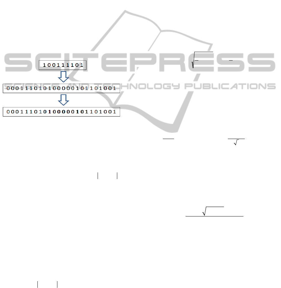
population. Figure 1 describes the random building

block operator.

Figure 1: The random building block operator. A random

building block is generated and copied to an individual to

produce a new offspring.

This operation is implemented in the following

order: 1) for each individual

ind two crossover

points

cp and

cp are randomly selected, 2) a

random bit string

bstr of length

cpcpl −=

generated, and 3) bits between the crossover points

on the individual

ind are replaced by the bit string

bstr . The following is the pseudo code for the

random building block operator.

procedure RandomBuildingBlock

begin

select individual from the population

select crossover point

[

)

)(,0

individuallengthcp ∈

select crossover point

[

)

)(,0

individuallengthcp ∈ so that

cpcp ≠ and

cpcp >

generate random bit string rbs of

length

cpcpl −=

replace bits between

cp and

cp on

the individual with rbs

Figure 2: The pseudo code for the random building block

(RBB) operator.

3.1 Survivor Selection

After each operator application, new offspring are

evaluated and compared to the population

individuals. Newly generated offspring will replace

the worst individual in the population if they are

better than the worst individual. Therefore, the

algorithm is a steady state genetic algorithm.

4 EXPERIMENTATION

The random building block operator was applied as

part of a genetic algorithm to solve the following

minimization problems:

The Ackley’s function:

⎟

⎠

⎞

⎜

⎝

⎛

∑

−

⎟

⎠

⎞

⎜

⎝

⎛

∑

−−+

).2cos(

exp

2.0exp2020

where

768.32768.32

≤

−

The Colville’s function:

22 2 22 2 2

21 1 43 3 2

424

100(x ) (1 ) 90( ) (1 ) 10.1(( 1)

( 1) ) 19.8( 1)( 1), where 10 10 for i 1,...4.

xxxxx x

xxx x

−

+− + − +− + − +

−+ − − −≤≤ =

The Griewank’s function F1:

1 100

( 100) cos( ) 1

4000

−

−+

∑∏

where

-600 x 600

≤

The Rastrigin’s function:

(10cos(2)10)

−+

∑

where

-5.12 x 5.12

≤

The Schaffer’s function F6:

22 2

sin 0.5

0.5

1.0 0.001( )

+−

⎡

⎤

⎣

⎦

where

100100

≤

−

For multidimensional problems with optional

number of dimensions (

n ), the algorithm was tested

for

50 ,10 ,5 3, ,2 ,1

The efficiency of the random building block operator

and three versions of single-point mutation operator

(with 1%, 5% and 8% mutation rates) and three

versions of multipoint mutation operator (with 5%,

8% and 15% mutation rates) in generating better

fitness values were tested separately 30 times for

each test case. The population size was set to 12 and

the maximum number of function evaluations for

ICEIS 2011 - 13th International Conference on Enterprise Information Systems

each run was set to 10,000. During each run the best

fitness value achieved during each generation was

recorded. This made it possible to figure out when

the best fitness value of the run was actually found.

Later at the end of 30 runs for each test case the

average of best fitness values and required function

evaluations were calculated for comparison. In the

following test results for comparing the random

building block operator with different versions of

mutation operator are reported.

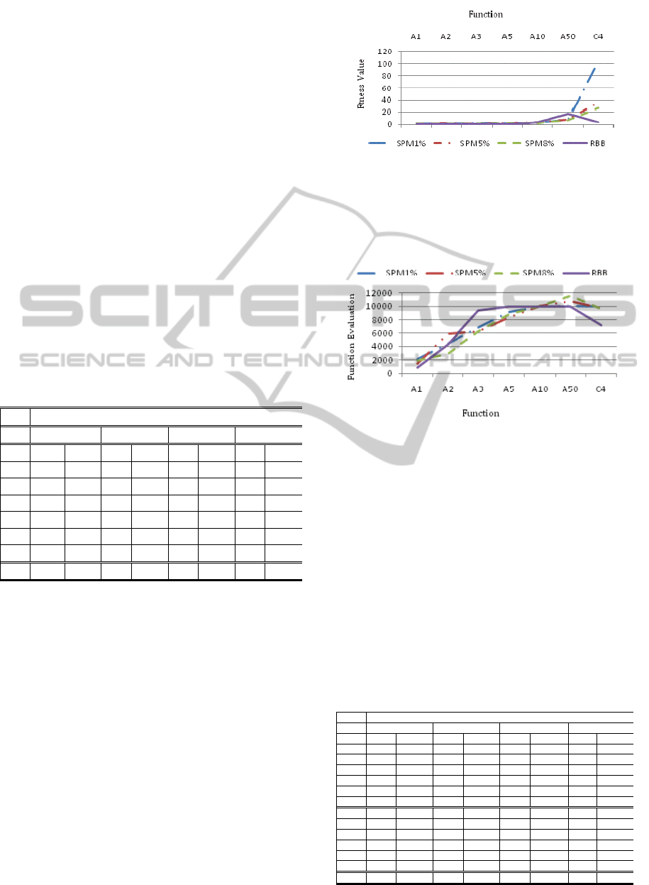
Table 1 summarizes test results for comparing

single-point mutation operator with the random

building block operator on Ackley’s and Colville’s

functions. In the table the average of best fitness

values and required function evaluations by single-

point mutation operator (with 1%, 5% and 8%

mutation rates) and the building block operator are

reported.

Table 1: Comparison of the average of the best fitness

values achieved for Ackley’s (A1-A50) and Colville’s

(C4) functions by single-point mutation (SPM) operator

with 1%, 5% and 8% mutation rates and the random

building block (RBB) operator. In the table Fn. stands for

function, F. for fitness and FE. for function evaluations.

Fn. Operator

SPM (1%) SPM (5%) SPM (8%) RBB

F. FE. F. FE. F. FE. F. FE.

A1 0.5 2097 0.2 1410 0.5 1927 0.0 889

A2 0.8 4399 1.5 5992 0.4 2896 0.0 4278

A3 1.5 6809 1.2 6275 1.2 6326 0.0 9400

A5 1.8 9127 1.5 8393 1.8 8863 0.0 10008

A10 2.3 10020 2.5 10146 2.0 10034 2.7 10008

A50 8.0 10146 7.6 10833 6.4 11550 16.9 10008

C4 103.9 10004 35.9 9793 26.7 9648 2.8 7225

Comparing results in Table 1 indicates that the

random building block operator has produced better

results than different versions of the single-point

mutation operator in 71% of test cases. In 14% of

test cases for Ackely’s function with 10 variables the

results were almost equal. But, the random building

block operator outperformed overwhelmingly on

Colville’s function. Figure 3 demonstrates

differences between average fitness values achieved

by different operators.

In many cases it took the random building block

operator less function evaluations to achieve better

fitness values and in some other cases it achieved

better fitness values than different versions of the

single-point mutation operator although more

function evaluations were required on average.

Figure 4 illustrates differences in the average

numbers of function evaluations.

Figure 3: Comparison of average fitness values achieved

for Ackley’s (A1-A50) and Colville’s (C4) functions by

the single-point mutation operator (with 1%, 5% and 8%

mutation rates) and the random building block operator.

The optimal fitness values for all functions are zero.

Figure 4: Comparison of the average numbers of function

evaluations needed by each operator to achieve the best

fitness values for Ackley’s (A1-A50) and Colville’s (C4)

functions.

The performance of the random building block

operator against the single-point mutation operator

was also tested on the Griewank’s, Rastrigin’s and

Schaffer’s F6 functions. Table 2 summarizes the test

results.

Table 2: Comparison of the average of the best fitness

values achieved for Griewank’s (G1-G50), Rastrigin’s

(R1-R50) and Schaffer’s F6 (S2 functions by single-point

mutation (SPM) operator with 1%, 5% and 8% mutation

rates and the random building block (RBB) operator. In

the table Fn. stands for function, F. for fitness and FE. for

function evaluations.

Fn Operator

SPM (1%) SPM (5%) SPM (8%) RBB

F. FE. F. FE. F. FE. F. FE.

G1 0.0 7566 0.0 6514 0.0 7552.4 0.0 2273

G2 0.6 10005 0.7 10028 0.7 9757 0.0 8771

G3 2.1 10008 2.2 10028 2.0 10015 0.0 10008

G5 3.8 10020 4.2 10015 3.8 10130 0.1 10008

G10 10.2 10028 10.4 10069 7.1 10008 1.5 10008

G50 62 10069 63 10234 56 11455 237 10008

R1 0.8 6570 1.3 7754 0.7 6200 0.0 431

R2 3.2 9732 3.4 9765 3.7 9473 0.0 2506

R3 7.7 10003 6.3 10029 6.2 9513 0.0 6500

R5 11.4 10000 11.8 10029 10.4 10188 0.0 10008

R10 24.4 10056 25.3 10139 24.6 10166 5.4 10008

R50 156 10139 157 10111 141 11549 313 10008

S2 0.2 8874 0.1 9218 0.2 9209 0.0 9222

RANDOM BUILDING BLOCK OPERATOR FOR GENETIC ALGORITHMS

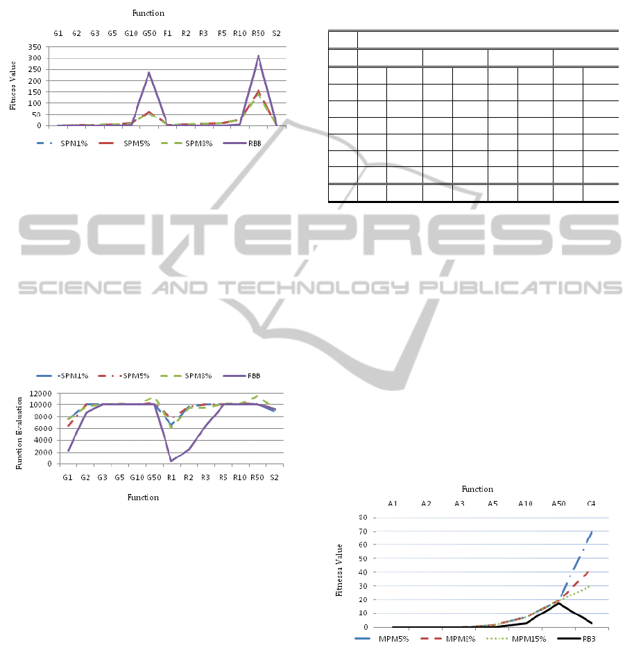
Studying data presented in Table 2 proves that the

random building block operator has been able to

produce significantly better results and in 85% of

test cases. Figure 5 illustrates the same results.

Figure 5: Comparison of the average of the best fitness

values achieved for Griewank’s (G1-G50) and Rastrigin’s

(R1-R50) functions with different variable numbers and

Schaffer’s F6 (S2) function by the single-point mutation

operator with 1%, 5% and 8% mutation rates (SPM1%,

SPM5% and SPM8%) and the random building block

(RBB) operator. The optimal fitness values for all

functions are zero.

The random building block operator achieved better

results in less function evaluations on average.

Figure 6 demonstrates differences in the average

numbers of function evaluations.

Figure 6: Comparison of the average numbers of function

evaluations needed on average by each operator to achieve

the best fitness value for Griewank’s (G1-G50),

Rastrigin’s (R1-R50) and Schaffer’s F6 (S2) functions.

The performance of the random building block

operator was also compared against the multipoint

mutation operator in which several points of the

individual were mutated during each mutation

operator. The number of points to be mutated during

each mutation operation was set to 2 times the

number of variables in the problem. This means that

if a problem had 5 variables, during each mutation

cycle, 10 points of the individual were randomly

selected to be mutated. Clearly, the total number of

mutation points was determined by the mutation

rate, which was 5%, 8% and 15% for different

experimentations.

Table 3: Comparison of best fitness values achieved for

Ackley’s (A1-A50) and Colville’s (C4) functions by

multipoint mutation (MPM) operator with 5%, 8% and

15% mutation rates and the random building block (RBB)

operator. In the table Fn. stands for function, F. for fitness

and FE. for function evaluations.

Fn. Operator

MPM (5%) MPM (8%) MPM (15%) RBB

F. FE. F. FE. F. FE. F. FE.

A1 0.0 6505 0.0 5249 0.0 4966 0.0 889

A2 0.0 10008 0.0 9817 0.0 9929 0.0 4278

A3 0.0 10008 0.0 10004 0.0 10032 0.0 9400

A5 1.1 10008 1.1 10004 1.3 10032 0.0 10008

A10 7.2 10008 6.9 10004 7.1 10032 2.7 10008

A50 19.2 10008 19.2 10004 19.2 10032 16.9 10008

C4 69.9 10000 43.1 9793 30.6 9648 2.8 7225

Comparing results reported in Table 3 proves that

the fitness values achieved by the building block

operator have been clearly better than the ones

achieved by different versions of the multipoint

mutation operator in all cases. Differences between

the average fitness values achieved for Colville

function by the random building block and different

versions of multipoint mutation operator are even

more substantial. The random building block

operator achieved an average fitness value of 2.7833

within average 7225 function evaluations, while the

multipoint mutation operator with 15% mutation rate

has achieved its best average fitness value of 26.66

within up to 9648 function evaluations. Figure 7

demonstrates differences between average fitness

values achieved by different operators.

Figure 7: Comparison of average fitness values achieved

for Ackley’s (A1-A50) and Colville’s (C4) functions by

the multipoint mutation (with 5%, 8% and 15% mutation

rates) and the random building block operator. The

optimal fitness values for all functions are zero.

Moreover, the best fitness values have been

achieved within less function evaluations with the

random building operator. Figure 8 depicts the

summary of differences in the number of function

ICEIS 2011 - 13th International Conference on Enterprise Information Systems

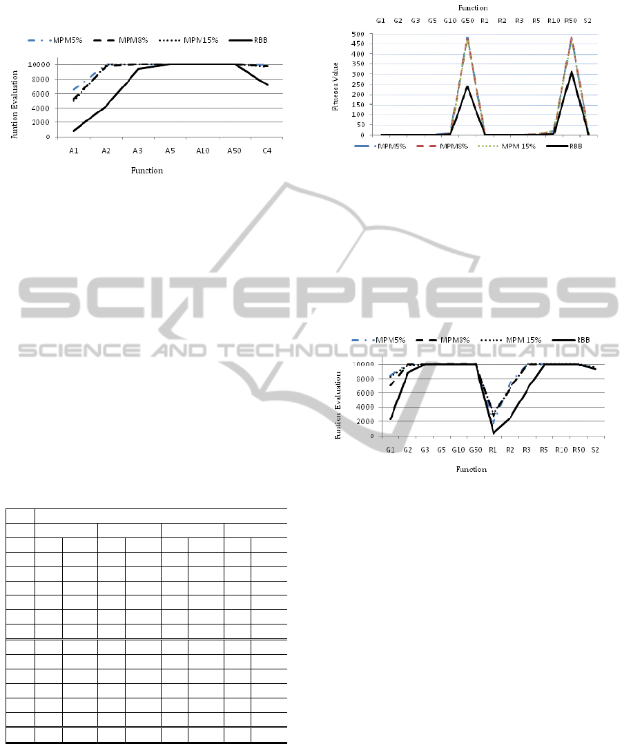
evaluations.

Figure 8: Comparison of the average numbers of function

evaluations needed by each operator to achieve the best

fitness values for Ackley’s (A1-A50) and Colville’s (C4)

functions.

As it can clearly be seen from Figure 8, the random

building block operator has in many cases needed

much less function evaluations to achieve the best

fitness values. The performance of the random

building block operator against the multipoint

mutation operator was also tested on Griewank’s,

Rastrigin’s and Schaffer’s F6 functions. Table 4

summarizes the test results.

Table 4: Comparison of the average of best fitness values

achieved for Griewank’s (G1-G50), Rastrigin’s (R1-R50)

and Schaffer’s F6 (S2) functions by multipoint mutation

(MPM) operator with 5%, 8% and 15% mutation rates and

the random building block (RBB) operator. In the table

Fn. stands for function, F. for fitness and FE. for function

evaluations.

Fn. Operator

MPM (5%) MPM (8%) MPM (15%) RBB

F. FE. F. FE. F. FE. F. FE.

G1 0.0 8490 0.0 7002 0.0 8253 0.0 2273

G2 0.0 10004 0.0 10008 0.0 9759 0.0 8771

G3 0.2 10004 0.1 10008 0.1 10008 0.0 10008

G5 1.0 10008 1.1 10014 0.9 10008 0.1 10008

G10 8.1 10008 6.1 10014 7.1 10008 1.5 10008

G50 479 10008 475 10014 468 10008 237 10008

R1 0.1 1768 0.2 2861 0.3 2973 0.0 431

R2 0.2 7341 0.2 6652 0.2 6630 0.0 2506

R3 0.3 10008 0.3 10008 0.3 10012 0.0 6500

R5 2.1 10008 2.3 10008 2.5 10012 0.0 10008

R10 22 10008 22 10008 22 10012 5 10008

R50 485 10008 485 1008 475 10012 313 10008

S2 0.0 9518 0.0 9383 0.0 9478 0.0 9222

Studying results presented in Table 4 proves that

compared to different versions of the multipoint

mutation operator, the random building block

operator has achieved better fitness values within

less function evaluations on average. These results

can also be observed from Figure 9.

Figure 9: Comparison of average fitness values achieved

for Griewank’s (G1-G50), Rastrigin’s (R1-50) and

Schaffer’s F6 (S2) functions by the multipoint mutation

operator with 5%, 8% and 15% mutation rates (MPM5%,

MPM8% and MPM15%) and the random building block

(RBB) operator. The optimal fitness values for all

functions are zero.

Figure 10 depicts the summary of differences in the

number of function evaluations.

Figure 10: Comparison of the average numbers of function

evaluations needed by each operator to achieve the best

fitness value for Griewank’s (G1-G50), Rastrigin’s (R1-

R50) and Schaffer’s F6 (S2) functions.

Figure 10 clearly indicates that compared to

different versions of multipoint mutation operator,

the random building block operator has needed less

function evaluations to achieve the best fitness

values on average.

5 CONCLUSIONS

In this paper a dynamic mutation operator; random

building block operator for genetic algorithms was

proposed. The operator was described and utilized in

solving five well-known test problems. The operator

was tested in 1020 runs for 34 test cases. For each

test case, the performance of the random building

block operator was tested against single-point

mutation operator with 1%, 5% and 8% mutation

rates and multipoint mutation operator with 5%, 8%

and 15% mutation rates. The maximum limit of the

RANDOM BUILDING BLOCK OPERATOR FOR GENETIC ALGORITHMS

function evaluations was set to around 10,000. Each

test case was repeated 30 times and the average of

the best fitness values and the average numbers of

function evaluations required for achieving the best

fitness value were calculated. Comparing test results

revealed that the random building block operator

was capable of achieving better fitness values within

less function evaluations compared to different

versions of single-point and multipoint mutation

operators. The fascinating feature of random

building block is that it is dynamic and therefore

does not require any parameterization. However, for

mutation operators the mutation rate and the number

of mutation points should be set in advance. The

random building block can be used straight off the

shelf without needing to know its best recommended

rate. Hence, it lacks frustrating complexity, which is

typical for different versions of the mutation

operator. Therefore, it can be claimed that the

random building block is superior to the mutation

operator and capable of improving individuals in the

population more efficiently.

5.1 Future Research

The proposed operator can be combined with other

operators and applied to new problems and its

efficiency in helping the search process can be

evaluated more thoroughly with new functions.

Moreover, the random building block operator can

be adopted as part of the genetic algorithm to

compete with other state-of-the-art algorithms on

solving more problems.

REFERENCES

Eiben, A. and J. Smith, 2007. Introduction to Evolutionary

Computing. Natural Computing Series. Springer, 2nd

edition.

Bäck, Thomas, David B. Fogel, Darrell Whitely & Peter

J. Angeline, 2000. Mutation operators. In:

Evolutionary Computation 1, Basic Algorithms and

Operators. Eds T. Bäck, D.B. Fogel & Z.

Michalewicz. United Kingdom: Institute of Physics

Publishing Ltd, Bristol and Philadelphia. ISBN

0750306645.

De Jong, K. A., 1975. An Analysis of the Behavior of a

Class of Genetic Adaptive Systems. Ph.D. thesis,

University of Michigan. Michigan: Ann Arbor.

Eshelman, L. J. & J.D. Schaffer, 1991. Preventing

premature convergence in genetic algorithms by

preventing incest. In Proceedings of the Fourth

International Conference on Genetic Algorithms. Eds

R. K. Belew & L. B. Booker. San Mateo, CA :

Morgan Kaufmann Publishers.

Eiben, G. and M. C. Schut, 2008. New Ways To Calibrate

Evolutionary Algorithms. In Advances in

Metaheuristics for Hard Optimization, pages 153–177.

Holland, J. H., 1975. Adaptation in Natural and Artificial

Systems. Ann Arbor: MI: University of Michigan

Press.

Mengshoel, Ole J. & Goldberg, David E., 2008. The

crowding approach to niching in genetic algorithms.

Evolutionary Computation, Volume 16 , Issue 3 (Fall

2008). ISSN:1063-6560.

Michalewicz, Zbigniew (1996). Genetic Algorithms +

Data Structures = Evolution Programs. Third,

Revised and Extended Edition. USA: Springer. ISBN

3-540-60676-9.

Michalewicz, Zbigniew, 2000. Introduction to search

operators. In Evolutionary Computation 1, Basic

Algorithms and Operators. Eds T. Bäck, D.B. Fogel &

Z. Michalewicz. United Kingdom: Institute of Physics

Publishing Ltd, Bristol and Philadelphia. ISBN

0750306645.

Mitchell, Melanie, 1998. An Introducton to Genetic

Algorithms. United States of America: A Bradford

Book. First MIT Press Paperback Edition.

Moghadampour, Ghodrat, 2006. Genetic Algorithms,

Parameter Control and Function Optimization: A New

Approach. PhD dissertation. ACTA WASAENSIA

160, Vaasa, Finland. ISBN 952-476-140-8.

Mühlenbein, H., 1992. How genetic algorithms really

work: 1. mutation and hill-climbing. In: Parallel

Problem Solving from Nature 2. Eds R. Männer & B.

Manderick. North-Holland.

Smit, S. K. and Eiben, A. E., 2009. Comparing Parameter

Tuning Methods for Evolutionary Algorithms. In IEEE

Congress on Evolutionary Computation (CEC), pages

399–406, May 2009.

Smith, R. E., S. Forrest & A.S. Perelson, 1993.

Population diversity in an immune system model:

implications for genetic search. In

Foundations of

Genetic Algorithms 2. Ed. L.D. Whitely. Morgan

Kaufmann.

Spears, W. M., 1993. Crossover or mutation? In:

Foundations of Genetic Algorithms 2. Ed. L. D.

Whitely. Morgan Kaufmann.

Ursem, Rasmus K., 2003. Models for Evolutionary

Algorithms and Their Applications in System

Identification and Control Optimization (PhD

Dissertation). A Dissertation Presented to the Faculty

of Science of the University of Aarhus in Partial

Fulfillment of the Requirements for the PhD Degree.

Department of Computer Science, University of

Aarhus, Denmark.

Whitley, Darrell, 2000. Permutations. In Evolutionary

Computation 1, Basic Algorithms and Operators. Eds

T. Bäck, D. B. Fogel & Z. Michalewicz. United

Kingdom: Institute of Physics Publishing Ltd, Bristol

and Philadelphia. ISBN 0750306645.

ICEIS 2011 - 13th International Conference on Enterprise Information Systems