THE CLASSIFICATION OF TIME SERIES UNDER THE

INFLUENCE OF SCALED NOISE

P. Kroha and K. Kr¨ober

Department of Computer Science, University of Technology Chemnitz, 09107, Chemnitz, Germany

Keywords:

Classiﬁcation, Market time series, Fractal analysis, Fuzzy technology, Stocks, Market behavior.

Abstract:

In this paper, we propose an improvement of a method for market time series’ classiﬁcation based on fuzzy

and fractal technology. Usually, the older values of time series will be cut off at a speciﬁc time point. We

investigated the inﬂuence of the fractal features on the classiﬁcation result. We compared a normal time series

representation, a representation having a smaller box dimension (achieved by exponential smoothing), and a

representation having a greater box dimension (achieved by addind scaled noise). We used different types of

noises and scales to improve the classiﬁcation result. Our application concerns time series of stock prices. The

market performance of those approaches is analyzed, discussed, and compared with the system without the

scaled noise component.

1 INTRODUCTION

There are two market hypotheses - the efﬁcient mar-

kets and the hypothesis of inefﬁcient markets. The

hypothesisof efﬁcient markets states that the informa-

tion obtained in the time series describing the stock

prices in the past is worthless to prediction because

the complete information from the past is already

fully evaluated, and contained in the last price value.

The hypothesis of inefﬁcient markets says that there

are some inﬂuences not completely evaluated, and re-

spected in the last price, and that these factors can be

used for prediction.

Since the beginning of stock trading, traders and

investors try to predict markets. One group of them

uses technical analysis that developed strategies to

analyse the behaviour of charts by means of techni-

cal indicators (e.g. moving average) and react ac-

cordingly, e.g. Turtle Trading (Faith, 2007). The

other group uses fundamental analysis that developed

strategies based on the economic data of companies

and markets, e.g. Value Investing (Graham, 2006).

We do not try to predict the markets. Our research

hypothesis is based on the hypothesis of inefﬁcient

markets and states that it is possible to classify se-

curities in such classes that some of them have sta-

tistically more chances to proﬁt in the current mar-

ket situation than the others. In our previous research

(Kroha and Lauschke, 2010), we implemented a sys-

tem based on fuzzy and fractal technology that sup-

ported our hypothesis stated above. Fuzzy clustering

and the Takagi-Sugeno inference method have been

used for processing of fractal features of time series.

In this paper, we investigate the inﬂuence of time

series fractal features to the classiﬁcation and describe

the implemented component. We analyze possibili-

ties of this method and compare it with the properties

of processes without this component by their average

performance.

The paper is structured as follows. In Section

2, we discuss the related works. Section 3 explains

shortly the concept of the fuzzy and fractal classiﬁer.

Sections 4 and 5 present why and how we extended

our previous system by different methods of noise

generation and exponential smoothing, and how we

scaled them. Experiments and data used are described

in Section 6. The evaluation and results are given in

Section 7 where we analyze all the approachesregard-

ing their market performance. Finally, we conclude in

Section 8.

2 RELATED WORKS

This paper introduces and investigates a method of

changing fractal features of time series added to ideas

published in our previouspaper (Kroha and Lauschke,

334

Kroha P. and Kröber K..

THE CLASSIFICATION OF TIME SERIES UNDER THE INFLUENCE OF SCALED NOISE.

DOI: 10.5220/0003442903340340

In Proceedings of the 6th International Conference on Software and Database Technologies (ICSOFT-2011), pages 334-340

ISBN: 978-989-8425-77-5

 2011 SCITEPRESS (Science and Technology Publications, Lda.)

2010) that explained also advantages of fuzzy and

fractal methods in comparizon to traditional methods.

A simple fractal system was published by Castillo

(Castillo and Melin, 2007). Compared to our sys-

tem, it uses a normal distribution of price differences

and does not use any changing of fractal features. In

our previous paper (Kroha and Lauschke, 2010), we

showed that the price differences are not normally dis-

tributed. Unfortunately, a direct comparison between

the two systems is impossible, because Castillo’s and

our system use different test environments (Castillo

and Melin, 2007).

Concerning fuzzy technology, there exist several

other applications of Takagi-Sugeno inference for

time series prediction. For example, the work of An-

dreu and Angelov (Andreu and Angelov, 2010), who

proposed an evolving Takagi-Sugeno algorithm for

time series prediction of NN GCI datasets. NN GCI

is a competition of classiﬁcation and prediction al-

gorithms. The key difference (aside from the data

they use), is that they use a different rule generation

method. They did not use c-mean clustering but linear

clustering. However, the reason why they used fuzzy

clustering is the same: to achieve data-based rule gen-

eration and to avoid static, upfront rulesets.

The ﬁeld of stock market prediction is ﬁlled with

hundreds of forecasting methods. Not all of those are

scientiﬁc or viable, but there exist several approaches

that are backed exactly. One example is the techni-

cal analysis that has also been tested as one of alter-

natives for generating input parameters for clustering

in our previous paper (Kroha and Lauschke, 2010).

Interestingly, in our experiments described in (Kroha

and Lauschke, 2010), the technical analysis module

performed worse than fractal analysis and the fuzzy

logic modules.

To classify the market type, we used a news-based

approach in (Kroha and Nienhold, 2010). We clas-

siﬁed stock market news stories into good, bad, and

neutral news and used then the ratio of these values

for prediction. We used the same approach in (Kroha

et al., 2010) but using a support vector machine for

the classiﬁcation.

We did not ﬁnd any previous works concerning the

fractal dimension changes suitable for classiﬁcation.

3 FUZZY AND FRACTAL

CLASSIFICATION

In this section, we will only very brieﬂy describe the

fuzzy and fractal features that we used in our sys-

tem (Kroha and Lauschke, 2010) before we introduce

the improvement by changing fractal dimension de-

scribed as our contribution in this paper. Our sys-

tem has the following three components: fractal di-

mension module, c-mean clustering algorithm, and

Takagi-Sugeno fuzzy inference module.

The fractal dimension module calculates the frac-

tal features of time series. They describe how chaotic

a given time series is. There are several ways to deﬁne

and calculate the fractal dimension. We used box di-

mension and Hurst coefﬁcient according to their def-

initions in (Mandelbrot, 1983). Details concerning

the fractal features of market can be found in (Peters,

1994) and in (Peters, 1996).

In addition, we had to use a correlation coefﬁcient

with a line to indicate whether the time series values

are going up or down.

A fuzzy classiﬁer uses three main components:

fuzzyﬁcation, fuzzy inference and defuzzyﬁcation.

The number of classes need to be deﬁned.

Fuzzyﬁcation is the process of transforming sharp

input data into fuzzy data using a membership func-

tion. The fuzzyﬁer determines what kind of cluster

is more probable for a given input value describing

the time series. The clustering algorithm c-mean dy-

namically calculates the membership function for the

fuzzyﬁcation process. As the input of the c-mean

clustering of time series, we used a triple consisting of

box dimension, Hurst coefﬁcient, and correlation co-

efﬁcient as mentioned above. Futher, it prepares data

for generation inferrence rules dynamically. More de-

tails can be obtained from (Castillo and Melin, 2003).

Then, using fuzzy inference according to the dy-

namically generated rules, a prediction value is in-

ferred. The rules are generated dynamically on the

basic of the input data. For this purpose, we used

the Takagi-Sugeno inference method (Kluska, 2009).

This function is valid for a certain dataset, it is, how-

ever, dynamic and individually generated for each

dataset.

To interpret the output prediction value, it will be

defuzziﬁed. In our case, its deﬁnition interval is di-

vided on three parts because we classify into three

classes. The prediction value membership to a subin-

terval indicates whether the classiﬁed time series will

be associated with the class BUY, SELL, or HOLD.

Time series of the class BUY have more common fea-

tures with time series that were going up in the past,

and time series of the class SELL have more common

features with time series that were going down in the

past under similar conditions. The architecture of our

time series classiﬁcation system is in Fig. 1.

THE CLASSIFICATION OF TIME SERIES UNDER THE INFLUENCE OF SCALED NOISE

335

Figure 1: Our time series classiﬁcation system.

3.1 Why Changing Fractal Dimension

Makes Sense

Supposing that a part of the future can be predicted

based on the history. Then the question is how much

of the history should be use to predict the future, and

whether all parts of the time series should have the

same weighting.

In stock market forecasting, there are many traders

who believe that older data is not as important as

newer data, e.g. daytraders. Other traders use some

indicators based on long time intervals, e.g. 20-day or

200-day simple moving average. Even though, some

features of a company are durable, many things can

change during 200 days. The administration of a com-

pany may change, its product may become obsolete,

new factories may be built that inﬂuence the price of

a product and competition on the market.

The ﬁrst version of our system was built on the

idea that inside of a speciﬁed time interval (we used

30 days for our experiments) each value of the time

series is as important as the other.

Classical methods of technical analysis usually

state a limit of the inﬂuence, they cut the inﬂuence

sharply (e.g. after 20 days, after 200 days), but all

values in the moving average have the same weight,

i.e. the same inﬂuence, like in the case of the simple

moving average.

There are also others models known, like

weighted moving average (more recent values are

more heavily weighted). The commonest type of

weighted moving average is exponential moving av-

erage applied as exponential smoothing. Exponen-

tial moving average (values are assigned to expo-

nentially decreasing weights over time) reacts faster

to recent prices and is used for known technical in-

dicator MACD (moving average convergence diver-

gence). Variable moving average is an exponential

moving average that derives its smoothing percentage

based on market volatility. Triangular moving aver-

age is double smoothed, i.e. it is averaged from sim-

ple moving averages. In such a case, investors using

these moving averages in their trading strategies must

have a special strategy for any kind of the moving av-

erage.

However, time is not the only one important fac-

tor. In (Kroha and Reichel, 2007), we classiﬁed tex-

tual market news using supervized learning, i.e. an

investor decided during the training phase which of

news stories is a good or bad story. When using

the trained and tested classiﬁer we stated that the ra-

tio of good stock market news to bad stock market

news build a context, e.g. investors are more enthu-

siastic, and has a predictive quality (Kroha and Nien-

hold, 2010). We experimented with time series fractal

features to inﬂuence the results of this classiﬁcation.

To decrease the box dimension we used exponential

smoothing, to increase the box dimension we used

added, scaled noise as we show in the next sections.

4 INCREASING FRACTAL

DIMENSION

Our original idea is to inﬂuence the fractal dimension.

To increase it we use noise. The key thoughts behind

this idea are:

• The addition of (random) noise to a part of time

series makes the time series more chaotic, result-

ing in appropriate fractal dimension changes.

• When noise is added to a time series with a very

distinct trend, the trend may penetrate through the

noise.

• Making a decision based on a noisy time series is

harder, therefore the algorithm will decide more

careful when a certain part of the time series is

noisy.

• If we now selectively noisify parts of the time se-

ries, e.g. the older parts, we enforce careful be-

havior by the algorithm. This selection we called

scaling the noise. It means that the noise ampli-

tude is controlled, scaled by a given function.

Figure 2: White noise.

ICSOFT 2011 - 6th International Conference on Software and Data Technologies

336

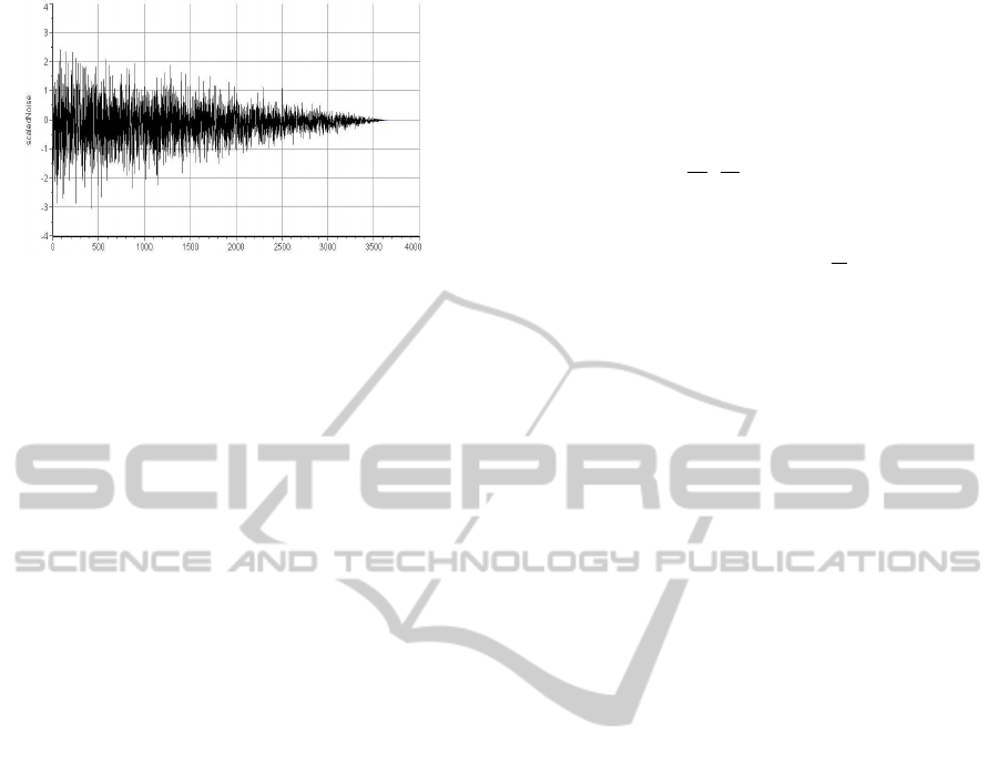
Figure 3: Scaled white noise.

Every noise variant is generated as a sequence

U = (u

,... ,u

). Every scaling variant is gen-

erated as a sequence S = (s

,... ,s

). They both

have the same size n, the size of the original time se-

ries X = (x

,... ,x

) for which they were gener-

ated. Now, we generate a new time series X

′

deﬁned

as (x

+ u

∗ s

+ u

∗ s

,...,x

+ u

∗ s

). In other

words, we scale the noise and add it to the time series.

There exist several different kinds of noise, which

differ by Hurst coefﬁcient. We chose to use white

noise for the ﬁrst version of our implementation be-

cause it is easy to generate and random. White noise

is a set of uncorrelated random variables with an ex-

pected value of zero and a constant variance. The ran-

dom values should be uniformely distributed. There

are several methods of generating white noise. We

chose to use the Central Limit Theorem (Kuo, 1996)

in our implementation.

The noise is used to inﬂuence the fractal calcula-

tions on the data, i.e. we do not inﬂuence the data

values. However, we do not want the whole time se-

ries to be noisy, just that parts that follow a certain

(predeﬁned) criteria, e.g. the older parts. Therefore,

as already described above, we had to scale the noise.

We decided to experiment with the noise scaled ac-

cording to linear function, Pareto function, and good

news/bad news function based on results in (Kroha

et al., 2006), (Kroha et al., 2007).

The scaling can be interpreted as a model of in-

ﬂuence probability of historical market prices on the

current price, i.e. the inﬂuence of older values weak-

ens accordingly to the scaling function.

Linear scaling takes the form of a linear function

with a dynamically adjusted gradient. The idea is,

that at the beginning of the time series (at time zero),

the linear function intersects the y-axis at exactly 1.

Precisely at the last point of the time series the lin-

ear function should reach 0. The scales are another

sequence of numbers with the same amount of data

points as the time series itself. The scales are deﬁned

as S = (s

,...,s

) with s

= 1− S∗ (1/n)∗ i or s

= 0

when the equation results in a number below 0. In the

equation S, there is a constant scaling parameter and

is used to inﬂuence the gradient of the linear function.

As basis for the Pareto scaling method, we use the

Pareto probability density function. It can be calcu-

lated as such:

(x) =

(

)

α+1

,α,x

> 0 (1)

α and x

are both parameters that can be chosen

freely. The Pareto density function equals 0 for all

x < x

. Then at x

it has the value of

. Afterwards it

declines rapidly and approaches 0 without ever reach-

ing it. Pareto scales can be heavily customized by

changing both the α and the x

parameter. Ideally, the

Pareto scales are ﬁtted for each time series, since this

cannot be done all the time, you need to ﬁnd parame-

ters that work for all your time series. For example, if

you would want to apply Pareto scales to a number of

time series, each consisting of 30 points, you would

need to set an x

in the interval [0,30]. Otherwise,

your Pareto scale values would be always 0 or near

zero.

As already discussed above, we wanted to in-

clude not only time dependent methods of scaling but

methods that use prefabricated prediction results from

other systems. As an example, we used our own im-

plemented method - a grammar-based prediction de-

rived from good and bad market news described in

(Kroha and Reichel, 2007).

5 DECREASING FRACTAL

DIMENSION

In the previous part, we described how to increase the

fractal dimension. In this section, we describe how to

decrease fractal dimension.

Exponential smoothing is a well known weighted

moving average for time series analysis. It is used

either for smoothing a time series to appear more aes-

thetically pleasing, or as a simple form of prediction,

based on past samples.

The calculation of a smoothened time series for an

input time series X = (x

,... ,x

) is done as such:

= x

(2)

= αx

+ (1− α) ∗ y

t− 1

,t > 1 (3)

α is the smoothing factor. If it is 1, each point of

the smoothened time series does not include informa-

tion of the past. When the value is near 0, the past

information is included to the fullest.

The basic idea of exponential smoothing and our

concept of changing fractal features of a time se-

ries using noise is similar. The smoothing process

THE CLASSIFICATION OF TIME SERIES UNDER THE INFLUENCE OF SCALED NOISE

337

Table 1: System without using noise.

variant 1 variant 2 variant 3

Box Dim 1.489 - 1.488

Hurst - 0.418 0.418

correlation 0.288 0.288 0.288

result 2.687 -13.040 0.731

decision 50 0 50

HOLD SELL HOLD

changes fractal features of a curve or a time series.

Older data points are assumed to have an exponen-

tially lesser inﬂuence on the future than newer ones

because of the member (1− α)

) in the deﬁnition. To

present smoothing like an addition of a noise compo-

nent we can imagine that smoothing adds a function

containing ”complementing asperities” to the time se-

ries so that the sum builds a smoothed curve.

6 USED DATA AND

EXPERIMENTAL RESULTS

We used the same input data as used in (Kroha and

Lauschke, 2010) to make it possible to compare the

two systems. This data consists of 53 stocks traded

in Germany. We chose to follow every stock from its

beginning onto the 21.07.2009, the day to which our

data extends. The trading strategy we used is from

our previous work (Kroha and Lauschke, 2010). Ev-

ery 30 days the program analyses this last timespan

(with and without noise) and makes a decision regard-

ing hold, buy or sell. Since our noise-based approach

is experimental, we have to ﬁnd out the difference to

the noise-free approach.

A calculation for each speciﬁc input variable com-

bination (box dimension, Hurst, correlation coefﬁ-

cient) takes around 20 minutes of computing time, re-

gardless of adding noise or not. We used a PC with the

following features - AMD Athlon Dual Core Proces-

sor 4850e, 2500 MHz (2 cores), 2 GB RAM, SAM-

SUNG SP2504C ATA hard disk.

6.1 Time Series without Changes

To test the existence of a difference, we used the

time series of the Adobe stock from 19.2.2001 to

30.3.2001, amounting to exactly 30 different data

points. There are three variants of possible input pa-

rameters. The ﬁrst variant consists of box dimension

and correlation coefﬁcient. The second variant con-

sists of Hurst Coefﬁcient and correlation coefﬁcient.

The third variant uses box dimension, Hurst coefﬁ-

cient and the correlation coefﬁcient.

Table 1 shows the input values of all three com-

binations obtained from the fractal method as well

as the y

res

decision value calculated by the Takagi-

Sugeno fuzzy inference for the Adobe time series.

The discrete decision value is calculated using a sim-

ple border test introduced in (Kroha and Lauschke,

2010). This means that in this particular case 1 all

variants suggest to hold, except the Hurst correlation

variant, which suggests to sell.

6.2 Increased Fractal Dimension

Now, we have to ﬁnd out what inﬂuence the addi-

tion of timescaled noise has on the parameters of

the process. The following experiment was done us-

ing scaled linear noise with a gradient of -2 over

the whole time series. That means at the beginning

the noise is the strongest and afterwards it declines

rapidly. At the middle point of the time series, the

noise stops completely. The decisions were SELL

(Variant 1), HOLD (Variant 2), and HOLD (Variant

3). The box dimension was shifted from 1.5 to 1.7. A

value near 2 means, the time series behaves randomly.

As expected, the addition of timescaled noise (which

is random) makes the time series more random. The

correlation coefﬁcient however, rises from 0.3 to 0.7

and therefore indicates a positive trend. The Hurst

Exponent is rather indecisive with a value near 0.5.

In the case of the news scaled white noise, the de-

cisions were HOLD (Variant 1), BUY (Variant 2), and

HOLD (Variant 3). This is the only test where the al-

gorithm actually proposed to buy stocks.

6.3 Decreased Fractal Dimension

The next experiment used an exponentially smoothed

time series, whereas α = 0.3. As expected, the

Hurst value changed in the direction of trends. Al-

though it is not a big change, the low smoothing fac-

tor only took out the sharpest edges of the time se-

ries. The Box Dimension changed accordingly. It de-

creased, which implies that the new time series con-

tains clearer trends. Correlation became more neu-

tral, it did not detect any positive or negative trends.

As one would expect, smoothing the time series takes

out some of the chaos, this can clearly be seen in the

newly calculated input values. The decisions were

HOLD (Variant 1), SELL (Variant 2), and HOLD

(Variant 3).

On the examples above, we just showed that the

decision signals change when applying scaled noise

on a time series of security prices. The next question

is whether it is in a common case of a time series the

same and how much performance, i.e. proﬁt, it brings.

ICSOFT 2011 - 6th International Conference on Software and Data Technologies

338

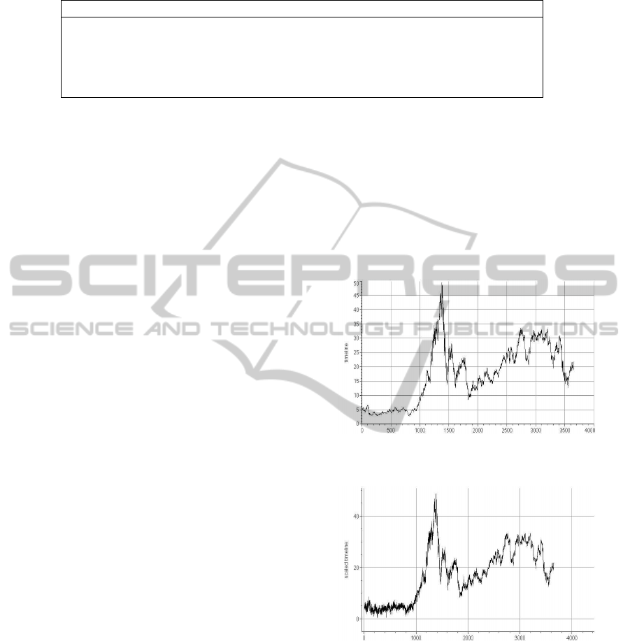
Table 2: Ranked results according to proﬁt earned.

rank proﬁt noise scale

1 175,537 exponential smoothing linear(factor 1)

2 174,386 none none - original values

3 167,688 white noise linear(factor 1)

4 142,388 white noise news controlled scale

5 112,040 none none - 10 day’s simple moving average

This topic is discussed in the next section.

7 EVALUATION AND ACHIEVED

RESULTS

To decide whether the change of fractal features has

brought any signiﬁcant changes in decision we have

to test how both methods perform in trading. Our ex-

periments and results are shown in this section.

When we try to classify the quality of a prediction

we have to think about the average case. The difﬁ-

culty is that in the stock market there is no average

situation against which a prediction algorithm could

be measured. So, we decided to process time series of

each of the 53 individual stocks and compare, which

approach performs best. We implemented a simula-

tion in which 10.000 Euros ares invested into each of

the 53 stocks at the beginning and we evaluate the re-

sults at the end of the time interval of 30 days.

The results of the test using the process without

noise show that it was proﬁtable in sum. The variant 1

of input parameters (box dimension/correlation) was

the most proﬁtable with a gain of 174,386. We ex-

perimented also with values of 10 day’s simple mov-

ing average. It leads to practically the same box di-

mension in each part of the time series, but its per-

formance is much worse 2 probably because of the

delay.

Increasing fractal dimension by a linear scaling

factor of 1 for linear scaled noise, the variant 3 ( box

dimension/Hurst/correlation) was the most proﬁtable

one, but with a gain only 167,688. Using factor 2, the

highest gain was 133,065. Using Pareto function (for

α = 0.3 and x

= 15), the highest gain was 128,395

for the variant 1. The experiment with news scaled

noise produced a good result, with a gain of roughly

142,000, it ranked 5 in the result comparison (see Ta-

ble 2). This shows that third party scales can be im-

plemented and used in our system.

Decreasing fractal dimension by exponential

smoothing without scaling was less promising. The

method achieved an (only average) gain of rougly

40000 in the ﬁrst two methods. Using box dimen-

sion, Hurst and correlation resulted in a loss of 1500.

Exponential smoothing seemed at ﬁrst sight as a good

method to include time information into the fractal

analysis, but performed subpar. We did another test

with linear scaled exponential smoothing. This exper-

iment showed a vast improvement over the unscaled

smoothing. With a gain of rougly 175,000 using vari-

ant 3 (box dimension/Hurst/correlation), this method

performed better than the original approach, if only

by a small amount.

Figure 4: Original time line - Adobe.

Figure 5: Time line with added noise - Adobe.

When dealing with the stock market, there were

several experiments that dealt with choosing stocks

randomly, e.g. using a monkey as an investor. We

also tried this approach to simulate randome deci-

sions. We did several tests, each with other random

number generator seeds. We found that the random

decision achieved a loss of 77,975 under the same

conditions. This means that it vastly underperformed

the fractal analysis approaches. None of the fractal

analysis methods made as big as a loss as the random

method.

THE CLASSIFICATION OF TIME SERIES UNDER THE INFLUENCE OF SCALED NOISE

339

Figure 6: Smoothened time line - Adobe.

8 CONCLUSIONS

As we can see in Table 2, the experiment based on ex-

ponential linear scaled exponential smoothing made

a greater proﬁt than the original approach without

scaled noise, i.e. decreasing fractal dimension inﬂu-

enced the classiﬁcation positively. In all cases, the

best combination of input values was used. It has

to be mentioned that real life trading has some ad-

ditional aspects. First, investors usually avoid some

stocks that do not have a promissing performance, so

they are not investing in all stocks and may achieve

statistically better performance. Second, we did not

involve fees and taxes paid when trading. This aspect

can worsen the performance very heavily.

However, there are several parameters in the gen-

eration and scaling of noise that can be tuned. For

example, using a time interval of only 20 days, we

obtained much less gain. So, much more experiment-

ing in the future is necessary.

Of course, we are aware of the fact that the pro-

cesses running behing the markets are sometimes

more, sometimes less chaotic, and because of that the

optimization of some features may fail.

Summarized, the answer to the question given in

our hypothesis at the very beginning is: Yes, fractal

dimension decreasing can improve the results at least

in some cases as shown above.

REFERENCES

Andreu, J. and Angelov, P. (2010). Forecasting time-series

for nn gc1 using evolving takagi-sugeno (ets) fuzzy

system with on-line inputs selection. WCCI 2010

IEEE World Congress on Computational Intelligence

CCIB, Barcelona, Spain.

Castillo, O. and Melin, P. (2003). Soft Computing and Frac-

tal Theory for Intelligent Manufacturing. Springer.

Castillo, O. and Melin, P. (2007). Evolutionary design and

applications of hybrid intelligent systems. Interna-

tional Journal of Innovative Computing and Applica-

tions Vol. 1, No. 1.

Faith, C. (2007). The Way of the Turtle: The Secret Methods

that Turned Ordinary People into Legendary Traders.

McGraw-Hill.

Graham, A. (2006). The Intelligent Investor. Collins Busi-

ness Essentials.

Kluska, J. (2009). Analytical Methods in Fuzzy Modeling

and Control. Springer.

Kroha, P., Baeza-Yates, R., and Krellner, B. (2006).

Text mining of business news for forecasting. In

In: Proceedings of 17th International Conference

DEXA’2006, Workshop on Theory and Applications of

Knowledge Management TAKMA’2006, pp. 171-175.

IEEE Computer Society.

Kroha, P., Kroeber, K., and Janetzko, R. (2010). Classiﬁ-

cation of stock market news using support vector ma-

chines. Proceedings of ICSOFT2010 - International

Conference of Software and Data Technologies, Vol.

1, pp. 331-336.

Kroha, P. and Lauschke, M. (2010). Using fuzzy and fractal

methods for analyzing market time series. Proceed-

ings of the International Conference of Fuzzy Com-

puting ICFC’2010, pp. 85-92.

Kroha, P. and Nienhold, R. (2010). Classiﬁcation of market

news and prediction of market trends. Proceedings of

the International Conference of Enterprise Informa-

tion Systems ICEIS’2010, Vol. 2, pp. 187-192.

Kroha, P. and Reichel, T. (2007). Using grammars

for text classiﬁcation. Proceedings of the Interna-

tional Conference of Enterprise Information Systems

ICEIS’2007, Vol. Artiﬁcial Intelligence and Decision

Support Systems, pp. 259-264.

Kroha, P., Reichel, T., and Krellner, B. (2007). Text mining

for indication of changes in long-term market trends.

In In: Tochtermann, K., Maurer, H. (Eds.): Proceed-

ings of I-KNOW’07 7th International Conference on

Knowledge Management as part of TRIPLE-I 2007,

Journal of Universal Computer Science, pp. 424-431.

Kuo, H.-H. (1996). White Noise Distribution Theory. CRC

Press.

Mandelbrot, B. (1983). Fractal Geometry of Nature. W.H.

Freeman, New York.

Peters, E. (1994). Fractal Market Analysis. Wiley.

Peters, E. (1996). Chaos and Order in the Capital Markets.

Wiley.

ICSOFT 2011 - 6th International Conference on Software and Data Technologies

340