
LEADER FOLLOWING FORMATION CONTROL FOR
OMNIDIRECTIONAL MOBILE ROBOTS
The Target Chasing Problem
Tiago Pereira do Nascimento, Fernando A. Fontes, Ant´onio Paulo Moreira
INESC Porto, Faculty of Engineering, University of Porto, Rua Dr. Roberto Frias s/n, 4200-465, Porto, Portugal
Andr´e Gustavo Scolari Conceic¸˜ao
Department of Electrical Engineering, Federal University from Bahia, Salvador, BA, Brazil
Keywords:
Formation control, Nonlinear model predictive controller, Mobile robots, Omnidirectional mobile robots.
Abstract:
This paper describes a novel approach in formation control for mobile robots. Here, a Nonlinear Model
Predictive Controller (NMPC) is used to maintain the formation of three omnidirectional mobile robots. The
details of the controller structure are presented as well as its functionality in a soccer robot team. Three Middle
Size League Robots are used for evaluation. A case of study based in a soccer robot situation is presented,
developed, and implemented to evaluate the performance of the controller. Simulations results are presented
and discussed.
1 INTRODUCTION
An adaptive framework based in predictive control for
creation and maintaining of a mobile robot team for-
mation was conceived as main objective of this work.
A formation is usually defined as the special arrange-
ment of a set of agents of the same type, where the
relative positions of its elements are steady even if
the formation is moving. The used formation differs
from the usual rigid formations where the relative po-
sition of a team element must be precisely maintained.
Here, the ideal formations are the ones that maximize
the team perception of the environment or of an ele-
ment that can be a leader robot or of a moving target.
A formation in ’V’ is usually normal in sets of
birds. This allows them to maximize the traveled dis-
tance and minimize the friction with the air flying in
the air tunnel left by the front bird. Nevertheless, in
the human sphere, a team formation can be used in
a variety of ways that goes from military operations
to team sports. In soccer for example, a formation
describes the number of players used in each tactic
formation in the field (defense, offense or middle). In
this sport, the formation is less rigid and highly dy-
namic.
The field of formation coordination and control of
a mobile robot team has been the area of many stud-
ies in recent years (Bicho et al., 2006), (Monteiro and
Bicho, 2008) and (Monteiro and Bicho, 2010). The
advantages of using a team of multiple robots include
robustness, flexibility, and adaptability to unknown
dynamic environments (Lim et al., 2009). These are
clearly important when considering applications such
as saving and rescue missions, deep ocean mapping,
forest fire detection, mine removal detection, or even
soccer robot competition.
In (Kanjanawanushkul and Zell, 2008) a strate-
gic division of formation control in three big groups
is made: leader following, virtual structure, and
behavior-based. There are also approximations purely
based in predictive control in which each robot has
an identical role in the formation. The virtual struc-
ture approach handles the problem as a rigid body
where all robots maintain a steady position, subjected
to physical constrains. In this strategy, any pertur-
bation made to any robot is propagated to the other
robots from the structure. This is due to a relatively
simple controller, as the ones described in (Tan and
Lewis, 1996), (Ghommam et al., 2010) and (Ren and
Beard, 2003). Nevertheless, the virtual structure ap-
proach has a high computational cost as the number of
robots increase. Another problem of this approach is
the velocity of the whole formation which is relatively
low, becoming a real problem in cases of dynamic ob-
135
Pereira do Nascimento T., A. Fontes F., Paulo Moreira A. and Gustavo Scolari Conceição A..
LEADER FOLLOWING FORMATION CONTROL FOR OMNIDIRECTIONAL MOBILE ROBOTS - The Target Chasing Problem.
DOI: 10.5220/0003453701350144
In Proceedings of the 8th International Conference on Informatics in Control, Automation and Robotics (ICINCO-2011), pages 135-144
ISBN: 978-989-8425-75-1
Copyright
c
2011 SCITEPRESS (Science and Technology Publications, Lda.)
stacle avoidance.
When using strategies based in a behavior-based
approach, reactive behaviors are used in each robot
to control formation integrated with other behaviors
used for trajectory tracking and obstacle avoidance
and detection. Good examples of this application can
be found in (Balch and Arkin, 1998), (Antonelli et al.,
2009) and (Liang and Xiao, 2010). The problem with
this approach is the description of the group dynamics
and the stability of the team.
Finally, the leader followingapproach is one of the
most studied. It is based on the existence of a leader
(real or virtual) robot that follows the precise desired
trajectory when the other robots of the formation just
follow it, maintaining a preset distance and relative
position. Most of these formation control strategies
employ predictive controllers.
An interesting application of the leader follow-
ing approach using Predictive Control is presented by
Zell and Kanjanawanishkull in (Kanjanawanushkul
and Zell, 2008). In this paper, the problem is solved
by dividing in two sub-problems essentially decou-
pled: the leader robot problem and the follower robots
problem. The leader robot follows a fixed trajectory
using a similar approach to (Kanjanawanushkul and
Zell, 2009), transmitting its velocity, state, and tra-
jectory to the other robots in formation. Therefore,
the followers use this information with the desired
formation to estimate its own reference trajectory.
Then, the follower robot follows this newly created
reference trajectory using the same controller used
by the leader. The formation problem proposed here
is decentralized, dividing the whole system in multi-
ple sub-systems which are independently controlled.
This allows the predictions horizons of control to be
bigger. Each robot solves its own optimization prob-
lem to follow its estimated trajectory.
The same authors presented in (Kanjanawanishkul
and Zell, 2008) another strategy to formation control
based in MPC, where each robot has to follow its own
reference trajectory while maintaining the desired for-
mation with the other robots of the group. It is as-
sumed that each robot has a pre-established reference
trajectory and that what the controller finds are the
velocities that each robot should have. In this case
the interaction between the formation robots is ac-
complished by coupling the cost function from the
controllers of each agent. Each robot solves locally
its control problem and passes the information to its
closest neighbors. Then, these robots solve their own
problem of minimization taking into account these
data in their cost function.
In (Fontes et al., 2009) a predictivecontroller with
two layers to control the formation of non-holonomic
mobile vehicles is proposed. It is considered that
there are two sub-problems to be solved to fulfill the
main objective: the trajectory control problem and the
formation control problem. With non-holonomic ve-
hicles, the problems are strictly different. When only
a single vehicle is moving to follow a fixed trajec-
tory it cannot move in any direction, therefore need-
ing a non-linear controller that would allow discon-
tinued feedback and control laws. However, when the
non-holonomic vehicle is moving as part of a forma-
tion, the relative position between the vehicles can be
modified in any direction as if they were holonomic.
To deal with this problem, only a linear controller was
needed.
It can be noticed that usually the state of the art
studies look for maintaining a rigid formation with
a robot team in which the relative positions between
the robots are fixed. This paper presents an approach
where the desired formation is not rigid. Therefore,
the proposed controller shall control the formations
that optimize the perception of the environment by the
team. By that, the robots relative positions have to
vary during the formation movement.
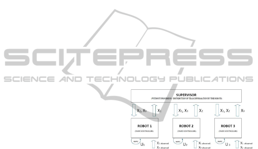
Figure 1: Distributed Architecture of a Distributed NMPC
Controller.
2 FORMATION CONTROL
The controller used in this work to formation con-
trol was a Non-linear Model Predictive Controller
(NMPC). The general structure of this controller can
be classified in three types: distributed, centralized,
or hybrid. These categories are based on the way the
control signals of each robot are calculated.
Here, the distributed architecture was chosen as
can be seen in Fig. 1. In this case, each one of the
robots calculates the total control inputs U
n
solving
its own optimization problem. This takes away the de-
pendencyfrom a central processing unit, guaranteeing
the functioning of the formation even in cases of com-
munication failure. Therefore, each robot must have
information about the state X
n
(position and speed) of
each mate of its team. Also, in case of the communi-
cation failure or supervisor failure, the robot uses its
ICINCO 2011 - 8th International Conference on Informatics in Control, Automation and Robotics
136
predicted open-loop strategy to determine these infor-
mations, having, therefore, a tolerance degree to fail-
ure. Nevertheless, it has the disadvantage of putting
a cost in computing the simulation of the entire for-
mation progression, which is done by each one of
the robots. However, this was not a problem, for the
robots only calculate their own control inputs. As
each robot solves its optimization problem in a decen-
tralized architecture, the formation becomes difficult
to stabilize.
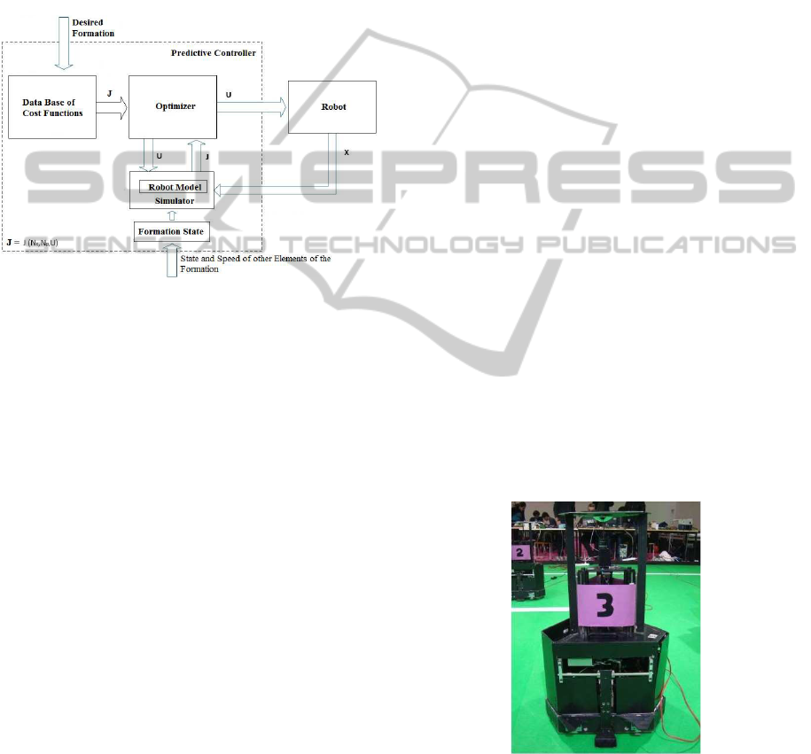
Figure 2: Structure of the Formation Controller Projected.
The capacity of the NMPC controller to create and
maintain a formation comes from the fact that cost
functions used by the controllers of each robot in the
team formation are coupled. This coupling is done
while the information about the position and speed of
the other robots are used in the cost function of each
robot to penalize the geometry or desired objective
deviation. This turns the entire group formation stable
where the actions of each robot affect the other mates.
Fig. 2 exposes the structure of the used controller.
This controller can be divided in three parts:
• State of the Formation - The controller contains
structures to keep the formations state (position
and speed of each other robot in the formation or
of any target that should be followed), updating
them in each control loop. These informations
can be received by a supervisor or by other robots
from the team, or even by the robot itself using its
own resources;
• Optimizer - This part uses a numeric minimiza-
tion method to optimize the cost function and ob-
tain the signals of optimal control. Here it is used
a method called Resilient Propagation (RPROP),
which guaranties quick convergence;
• Simulator - This part does the simulation not
only of the robot state evolution but also the state
evolution of the other elements in the formation
(other robots or targets). This element uses a dy-
namic simplified model to emulate the robot evo-
lution. The speeds of the other robots or targets
are assumed during the entire horizon of predic-
tion as being constant and equals to the actual
speed.
The controller receives as parameters the desired
formation, the position of the robot in formation and
the actual state of the other elements in the formation.
For each formation there are a differentcost functions.
Then each mDec uses its controller optimizer and it
starts to give to the simulator the control input U for
the robot the mDec is controlling. The simulator uses
this information to simulate the complete formation
evolution for the prediction horizons T
p
. The simu-
lator gives back to the optimizer a cost value to the
control inputs, and the iterative process of minimiza-
tion is repeated cyclic.
The Resilient Propagation algorithm (RPROP) ap-
peared in the learning algorithms category used in
neural networks (Riedmiller and Braun, 1993), be-
ing adapted to this application. This is an adaptive
method where the step value is not proportional to
the gradient function value to be minimized in a de-
sired point (as it happens in the Steepest Descent al-
gorithm), but it keeps adapting with the function be-
havior. Therefore, it becomes immune to the uncer-
tainties of the derivative function value, depending
only on the temporal behavior of its signal. This algo-
rithm was tested initially with the values suggested by
(Riedmiller and Braun, 1993) (η
+
= 1.5, η
−
= 0.5,
∆
0
= 0.1) and it revels to be capable to converge
where the Steepest Descent failed.
Figure 3: The 5DPO Robot.
3 PROBLEM FORMULATION
The developed framework was applied to a forma-
tion with three omnidirectional mobile robots from
LEADER FOLLOWING FORMATION CONTROL FOR OMNIDIRECTIONAL MOBILE ROBOTS - The Target
Chasing Problem
137
the FEUP’s 5DPO team (Fig. 3) that can fulfill two
main objectives: the optimization of the target relative
velocity perception and relative state perception (ball
relative velocity perception and relative state percep-
tion) using two robots (observers) while a third robot
places itself in an ideal position to receive the ball (re-
ceiver). The robots should maintain this formation
following the ball movement and avoiding the colli-
sions between them or with the target.
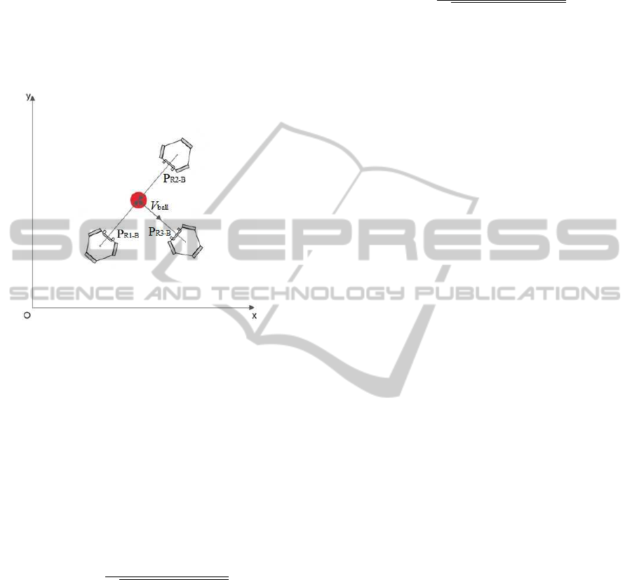
Figure 4: The Desired Formation.
The mathematical definition of the system can be
understood as having three robots and a ball (target).
Taking as base for this formation definition the ele-
ments presented in Fig. 4. The ball position and speed
vectors in global coordinates are respectively:
X
ball
(k) =
x
ball
(k) y
ball
(k)
T
, (1)
v
ball
(k) =
vx
ball
(k) vy
ball
(k)
T
. (2)
It is considered also that the unit vector of the
ball’s velocity ˆv
ball
(k)=[ ˆvx
ball
(k), ˆvy
ball
(k)]
T
, is such
that:
ˆv
ball
(k) =
v
ball
(k)
q
vx
2
ball
(k) + vy
2
ball
(k)
. (3)
For each robot n, its state is represented by:
X
n
(k) =
x
n
(k) y
n
(k) θ
n
(k)
T
, (4)
V
n
(k) =
vx
n
(k) vy
n
(k) w
n
(k)
T
. (5)
The position of the ball with respect to robot n is
given by P
Rn−B
(k)=[x
Rn−B
(k), y
Rn−B
(k)], where:
P
Rn−B
(k) =
(x
ball
(k) − x
n
(k)) (y
ball
(k) − y
n
(k))
.
(6)
Then, it shall be defined the unit vector
ˆ
P
Rn−B
(k)=[ ˆx
Rn−B
(k), ˆy
Rn−B
(k)], which indicates the
direction of the ball with respect to the robot, and its
angle θ
Rb−B
:
ˆ
P
Rn−B
(k) =
P
Rn−B
(k)
q
x
2
Rn−B
(k) + y
2
Rn−B
(k)
, (7)
θ
Rb−B
(k) = atan2(y
Rn−B
(k), x
Rn−B
(k)). (8)
Finally, there is also the definition of the positions of
each robot n with respect to its mates in the formation
y, given by P
Rn−Ry
(k)=[x
Rn−Ry
(k), y
Rn−Ry
(k)], where:
P
Rn−Ry
(k) =
(x
n
(k) − x
y
(k)) (y
n
(k) − y
y
(k))
.
(9)
3.1 The Observer Robot
The estimation of the quality of the ball state is a func-
tion of its moving direction with respect to the robot
and the distance in between. This estimation is done
by using a omnidirectional vision system, the descrip-
tion of which can be found in (Gouveia, 2008). There-
fore, it’s clear that in this case, the robot’s direction is
irrelevant.
Nevertheless, big distances between the robot and
the ball results in failure of the ball’s detection. Con-
sequently, this leads to the failure to estimate its ve-
locity. When the distance is too small, it can occur
that the robot cannot see the entire ball and, therefore,
become incapable to detect correctly its position in-
creasing the risk of undesired collisions. Take as an
example the case in which the distance between the
ball and the robot decreases with time in a straight
line. In this case the robot only sees the ball increas-
ing in size, making it difficult to estimate its velocity.
In the ideal case the ball should move perpendicular
to its position with respect to the robot. Therefore, the
desired formation for the observer robots to be around
the ball in a way to better estimate the ball velocity
possesses the following characteristics:
• Each one of the robots puts itself in opposite sides
of the ball, maintaining a parallel velocity with
respect to the ball, v
ball
, with the same modulus;
• The robot position vector with respect to the ball,
P
Rx
B
, must be perpendicular to the ball’s velocity
vector, v
ball
;
• Each one of the robots must maintain a distance
|P
Rx
B
| from the ball;
• The robots must not collide between them.
Therefore, taking into account all the elements
previously described, the weights given to each one
of them, and a penalization term to the variation of
control effort, the cost function that represents all this,
ICINCO 2011 - 8th International Conference on Informatics in Control, Automation and Robotics
138

embedded in each of the two observer robots is as fol-
lows:
J(N
1
, N
2
, N
c
) =
N
2
∑
i=N
1
λ
1
(d
setpoint
− |P
Rn−B
(i)|)
2
+
N
2
∑
i=N
1
λ
2
(
ˆ
P
Rn−B
(i) · ˆv
ball
(i))
2
+
N
2
∑
i=N
1
λ
3
((
1
−d
min
+ |P
Rn−Rm
1
(i)|
)
2
+
(
1
−d
min
+ |P
Rn−Rm
2
(i)|
)
2
)+
N
c
∑
i=1
λ
4
(∆U(i))
2
,
(10)
Where,
• N
1
, N
2
- prediction horizon limits, in discrete time,
so that N
1
> 0 e N
2
≤ N
p
, where N
p
is the desired
prediction horizon.
• N
c
- control horizon.
• λ
1
, λ
2
, λ
3
, λ
4
- weights for each component of the
cost function
• ∆U(k) = [v
r
(k) − v
r
(k − 1)] + [vn
r
(k) − vn
r
(k −
1)] + [w
r
(k) − w
r
(k− 1)] - variation of the control
signals, with U(i) being the reference velocities
vector with respect of the center of mass of the
robot.
3.2 The Receiver Robot
The ideal position of the receiver robot with respect to
the ball to have a good reception of it corresponds to
the one in which the robot velocity vector is collinear
with the ball velocity vector, with the same modu-
lus. Also, the robot orientation should be such that the
front of the robot is turn towards the ball. Therefore,
the robot can then slowly decelerated and the distance
between it and the ball can be decreased in a way to
receive the ball in ideal conditions.
Summarizing it, theformation here should possess
the following characteristics:
• The robot’s velocity has to be equal in modulus
and direction to the ball’s velocity v
ball
;
• The robot’s position vector with respect to the
ball, P
Rn−B
, must be collinear to the ball’s velocity
vector, v
ball
;
• The robot’s orientation θ
n
must be at all times
equal to the vector P
Rn−B
’s angle, defined by
θ
Rn−B
, in a way that the kicker of the robot is al-
ways turn towards the ball;
• The robot must be at a distance |P
R−B
| from the
ball.
Finally, joining all the elements previously de-
scribed, the weights given to each one of them, and
a penalization term to the variation of control effort,
the cost function that represents all this, embedded in
the receiver robot is as follows:
J(N
1
, N
2
, N
c
) =
N
2
∑
i=N
1
λ
1
(d
setpoint
− |P
Rn−B
(i)|)
2
+
N
2
∑
i=N
1
λ
2
(−1)
2
+
N
2
∑
i=N
1
λ
3
((
1
−d
min
+ |P
Rn−Rm
1
(i)|
)
2
+
(
1
−d
min
+ |P
Rn−Rm
2
(i)|
)
2
)+
N
2
∑
i=N
1
λ
4
(dif fAngle(θ
n
, θ
Rn−B
))
2
+
N
c
∑
i=1
λ
5
(∆U(i))
2
,
(11)
Where,
• N
1
, N
2
- predictionhorizon limits, in discreet time,
so that N
1
> 0 e N
2
≤ N
p
, where N
p
is the desired
prediction horizon.
• N
c
- control horizon.
• λ
1
, λ
2
, λ
3
, λ
4
, λ
5
- weights for each component of
the cost function
• ∆U(k) = [v
r
(k) − v
r
(k − 1)] + [vn
r
(k) − vn
r
(k −
1)] + [w
r
(k) − w
r
(k− 1)] - variation of the control
signals, with U(i) being the reference velocities
vector with respect of the center of mass of the
robot.
4 RESULTS
Once the formation algorithm was implemented,
some tests in simulation were made to validate the
proposed controller and to test its performance un-
der different conditions. Here, a simulation software
called SimTwo was used to simulate the formation
(Costa, 2010) done by three omnidirectional robots
and the target (ball).
In this simulation the SimTwo has the job of an-
other software called HAL (Hardware Abstraction
Layer), which is an application that receives the sen-
sor signals and communicates with the actuators, and
LEADER FOLLOWING FORMATION CONTROL FOR OMNIDIRECTIONAL MOBILE ROBOTS - The Target
Chasing Problem
139
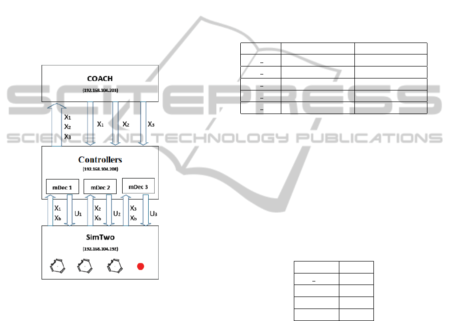
then with the mDec (software of control of the real
robots) by IP protocol. In the real robots, the HAL
sends to the robot’s mDec the state of the other robots
and the state of the ball. Then, each mDec sends to
the SimTwo the control references of its robot. Each
mDec also communicates with another central com-
puter (the supervisor) that contains the Coach soft-
ware, sending its own state and the state of the ball
while observing it. Finally, the Coach sends to each
mDec individually the state of the other robots in for-
mation, in a way that each robot has the information
of position and velocity of its mates. It can be noticed
that this arrangement is similar the one used in real
experiments, where the only difference is the replace-
ment of the SimTwo for the HAL in each robot.
Figure 5: Communications between applications diagram.
There are many variables that influences the qual-
ity of the result. Among them are the weights (the
λ
i
) of each cost function and the optimizer parame-
ters. The cost function values for both observer and
receiver robots can be seen in table 1. In the min-
imization of the cost function values, only the rela-
tionship between the weights given to each element
that meters to the final result. Therefore, to the penal-
ization of the relative position with respect to the ball
λ
2
was given a value ten times bigger than the penal-
ization of the distance between the robot and the ball
λ
1
, due to the fact that the first penalization is harder
to maintain. The weight given to the penalization of
the proximity between robots, λ
3
, was set very high to
avoid the maximum number of collisions. The penal-
ization for the receiver robot’s orientation, λ
4
in table
1, was set as half of λ
2
, for this was not very impor-
tant to the formation. Finally, the value of the control
effort (λ
4
in the first table and λ
5
in the second one)
was chosen to be the smallest value that could forbid
the robots to move themselves around the target when
this was stationary. The final values were a result of
an iterative process. This process did not need to be
very precise, due to the fact that there were a very
large range of weights that could give similar results.
Nevertheless, the NMPC controller parameters were
N
p
= 10, N
c
= 2 and the used reference trajectory to
find them was an gate signal extracted in a previous
work done by (Ferreira and Moreira, 2010).
Table 1: Weights for the Observers and Receiver.
Weight Observer Value Receiver Value
λ 1 10 10
λ 2 100 100
λ 3 100 100
λ 4 5 50
λ 5 - 5
The initial parameters used on the RPROP opti-
mization algorithm were the ones suggested by (Ried-
miller and Braun, 1993) where the algorithm descrip-
tion can also be found. The fist tests were done with
these parameters (η
+
= 1.5 and η
−
= 0.5) and re-
sulted in a very satisfactory performance by the con-
troller. Some changes made on these values were
tested (decrement of η
+
and increment of η
−
) and
produced visible improvements, having the final val-
ues become as the ones shown in table 2.
Table 2: RPROP optimizer parameters.
Variable Value
IT max 20
ε 0.05
η
+
1.2
η
−
0.8
Therefore, the following simulation results made
with the formation control framework evaluate the
proposed controller. First, the simulations for forma-
tion convergence are shown to evaluate the formation
controller. Secondly, simulations for the evaluation of
the formation maintenance were made.
4.1 Formation Convergence Results
The following results show the trajectories followed
for each one of the robots when, starting from dif-
ferent positions, converge to a preset formation. The
target in these cases is stationary during the simula-
tion making the internal product of any vector with
the ball velocity vector equals to zero. It is impor-
tant to notice that the robots number 1 and 2 are the
ICINCO 2011 - 8th International Conference on Informatics in Control, Automation and Robotics
140
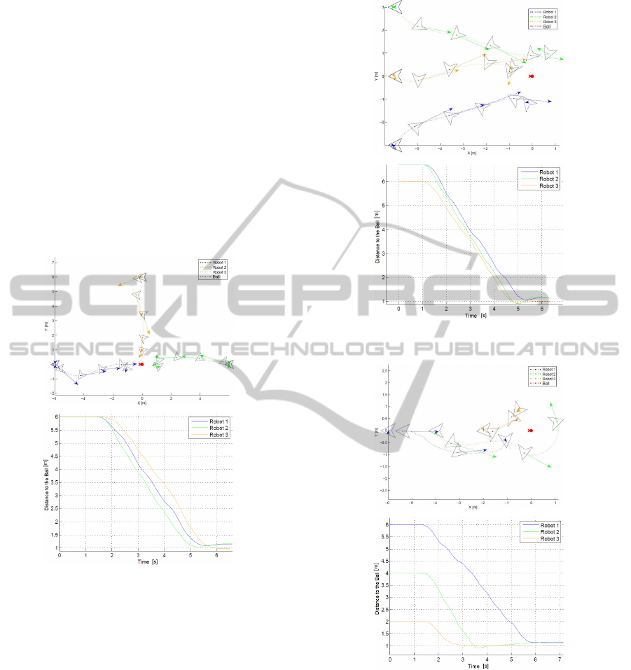
observer robots while the robot number three is the re-
ceiver robot. The desired distance between each robot
to the ball was defined to be 1 m.
4.1.1 Simulation 1
In this simulation the robots start at positions per-
fectly opposites and far from the ball. For having less
risk of collision or probability of the robots to inter-
fere with each other, this became the simplest case.
The results can be seen in Fig. 6. The robots con-
vergeperfectly to their positions in formation, making
straight trajectories towards the target. As can be seen
in the plot of the distance with respect to the time, it
can be estimate that the robots have converged to the
desired formation in approximately four seconds.
Figure 6: Convergence into formation, simulation 1.
4.1.2 Simulation 2
Here all robots start from the same side of the ball,
thought separated by a distance of 3 m. The results
can be seen in Fig. 7. From this simulation on it can
be noticed some interaction between the robots. The
robot 3 went directly to the ball, in a straight line.
The robots 1 and 2 went also to the ball avoiding the
robot 3 when starting to get close to this robot. This
formation converged in about 5 seconds.
4.1.3 Simulation 3
The third simulation shows a more complex situation,
where the robots start from the same alignment with
respect to the ball. The results can be seen in Fig.
8. The robot 3, closest to the ball, went to occupy
Figure 7: Convergence into formation, simulation 2.
Figure 8: Convergence into formation, simulation 3.
instantaneously the position in its front. When the
robot number 2 approaches the ball, the robot number
3 moves slightly up, therefore, going around the ball,
and occupying the space behind it. Finally, the robot
number 1 puts itself in the space left by robots number
2 and 3. This process takes about 4.5 seconds.
LEADER FOLLOWING FORMATION CONTROL FOR OMNIDIRECTIONAL MOBILE ROBOTS - The Target
Chasing Problem
141
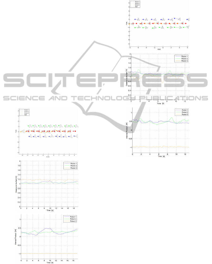
4.2 Formation Maintenance Results
Now, the following simulations test situations in
which, once the formation is made, the robots must
maintain it moving in formation while tracking the
target (the ball). These simulations were made to
evaluate the capacity of the controller to maintain the
desired formation. Besides the XY plot and the dis-
tance with respect to time graph, the graph of the in-
ternal product between the ball velocity vector and the
each robot position vector with respect to the ball was
also shown.
4.2.1 Simulation 1
In these testes the target moved in a straight line
trajectory with a constant velocity that varied from
0.5m/s to 1.5m/s. These simulations can be seen in
Figs. 9, 10, and 11. This is the simplest situation to
maintain the formation in a target tracking problem,
given the fact that the target velocity has direction and
velocity constant what allows the controller to predict
exactly its progression.
Figure 9: Maintaining formation in a straight line, simula-
tion 1a.
To the target velocity equals to 0.5m/s and 1.0m/s
the performance of the controller is similar and
presents an acceptable accuracy. The distances from
Figure 10: Maintaining formation in a straight line, simula-
tion 1b.
the ball are maintained close to the desired vale of
1 m while the values of the internal product are also
similar to the desired ones (0 to the robots 1 and 2
and -1 to the robot 3). It can be noticed in the graphs
of internal product, that the internal product of two
unit vectors vary much more quickly around 0 then
around -1. Therefore, the bigger variations of the in-
ternal product in robots 1 and 2 do not mean a bad
control (as it can be seen in the plots XY).
With a velocity of 1.5m/s the controller shows
a little difficulty in maintaining the formation with
accuracy. The robots 1 and 2, although a little bit
late with respect to the ball, do succeed in main-
taining the desired formation. However, the robot 3
presents some difficulty in following the target trajec-
tory, putting itself closer than it should what made it
oscillate around the desired one.
ICINCO 2011 - 8th International Conference on Informatics in Control, Automation and Robotics
142
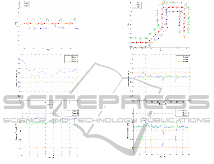
Figure 11: Maintaining formation in a straight line, simula-
tion 1c.
4.2.2 Simulation 2
This last simulation had the objective to evaluate the
behavior of the controller when the target changes
its direction abruptly. It has also the objective to
evaluate if the robots are capable of reset their for-
mation positions correctly avoiding any collision be-
tween them. For that porpoise, two types of corners
were tested: a 135
o
corner (a less abrupt angle) and a
90
o
corner (or a right angle). The results can be seen
in Fig. 12 using a speed of 0.5m/s.
By each change of direction the entire formation
turns around the target and the robots reset their posi-
tion in formation in a way to occupy the correct posi-
tions. Observing the plots of distance with respect to
the time and internal product with respect to the time,
the formation takes about three seconds to reset.
5 CONCLUSIONS
In this paper a novel approach of a Non-linear Model
Figure 12: Maintaining formation in a corner trajectory,
simulation 2a.
Predictive Controller was presented to formation con-
trol of omnidirectional mobile robots. The devel-
oped framework showed to be very flexible and eas-
ily adaptable. The projected controller is capable of
making the team of robots to converge to the de-
sired geometry around a target, even if the robots
are very far apart. The merit of this accomplishment
can be directed to the minimization algorithm used,
the RPROP. Also, due to the high penalization on
the extreme proximity between robots, the collisions
between them are effectively limited or completely
avoided.
In terms of maintaining the formation, the ob-
tained results are highly dependent of the target veloc-
ity characteristics. In low velocities the results were
obviously better due to the fact that the errors from the
incorrect predictions do not result in big deviations in
the desired geometry as it does when the velocities
are high. In general, the controller reacted well to
abrupt changes in the target speed direction, with the
formation circulating the target instantaneously after
the change in direction. Consequently, it made the ge-
ometry to be reset to accommodate the new direction.
LEADER FOLLOWING FORMATION CONTROL FOR OMNIDIRECTIONAL MOBILE ROBOTS - The Target
Chasing Problem
143

ACKNOWLEDGMENTS
The authors thank the INESC Porto for contributing
to this work and to the FCT (Fundac¸˜ao para Ciˆencia e
Tecnologia) from Portugal for supporting the project
PTDC/EEA-CRO/100692/2008 - ”Perception-Driven
Coordinated Multi-Robot Motion Control”.
REFERENCES
Antonelli, G., Arrichiello, F., Chiaverini, S., and Cassino, S.
(2009). Experiments of Formation Control With Mul-
tirobot Systems Using the Null-Space-Based Behav-
ioral Control. IEEE Transactions on Control Systems
Technology.
Balch, T. and Arkin, R. C. (1998). Behavior-based forma-
tion control for multirobot teams. IEEE Transactions
on Robotics and Automation.
Bicho, E., Diegues, S., Carvalheira, M., Moreira, A. P.,
and Monteiro, S. (2006). Airship Formation Con-
trol. In Proceedings of the 3rd Int. Conf. on In-
formatics in Control, Automation and Robotics, in
Workshop Multi-Agent Robotic Systems (MARS 2006),
pages 22–33.
Costa, P. J. (2010). Simtwo. Available from http://paginas.
fe.up.pt/∼paco/wiki/index.php?n= Main.SimTwo.
Ferreira, J. R. and Moreira, A. P. G. M. (2010). Non-linear
Model Predictive Controller for Trajectory Tracking
of an Omni-directional Robot Using a Simplified
Model. In 9th Portuguese Conference on Automatic
Control.
Fontes, D. M., Fontes, F. A., and Caldeira, A. (2009). Model
Predictive Control of Vehicle Formations. Optimiza-
tion and Cooperative Control Strategies, M.J. Hirsch,
C.W. Commander, P. Pardalos, and R. Murphey ed-
itors, Lecture Notes in Control and Information Sci-
ences, Springer Verlag.
Ghommam, J., Mehrjerdi, H., Saad, M., and Mnif, F.
(2010). Formation path following control of unicycle-
type mobile robots. Robotics and Autonomous Sys-
tems.
Gouveia, M. C. M. (2008). Estudo e implementac¸ ˜ao
de um algoritmo de localizac¸˜ao baseado em corre-
spondˆencia de mapas. Master Thesis in Electronic
and Computers Engineering, Faculty of Engineering
from University of Porto.
Kanjanawanishkul, K. and Zell, A. (2008). Distributed
model predictive control for coordinated path follow-
ing control of omnidirectional mobile robots. In IEEE
International Conference on Systems, Man and Cy-
bernetics, 2008. SMC 2008, pages 3120–3125.
Kanjanawanushkul, K. and Zell, A. (2008). A model-
predictive approach to formation control of omnidi-
rectional mobile robots. In Intelligent Robots and Sys-
tems, 2008. IROS 2008. IEEE/RSJ International Con-
ference on, pages 2771–2776.
Kanjanawanushkul, K. and Zell, A. (2009). Path following
for and omnidirectional mobile robot based on model
predictive control. In 2009 IEEE International Con-
ference on Robotics and Automation.
Liang, X. and Xiao, Y. (2010). Studying bio-inspired coali-
tion formation of robots for detecting intrusions using
game theory. IEEE transactions on systems, man, and
cybernetics: Part B.
Lim, H., Kang, Y., Kim, J., and Kim, C. (2009). Forma-
tion control of leader following unmanned ground ve-
hicles using nonlinear model predictive control. In
Advanced Intelligent Mechatronics. IEEE/ASME In-
ternational Conference on AIM 2009.
Monteiro, S. and Bicho, E. (2008). Robot formations:
robots allocation and leader-follower pairs. In Pro-
ceedings of the 2008 IEEE International Conference
on Robotics & Automation (ICRA2008), pages 3769–
3775.
Monteiro, S. and Bicho, E. (2010). Attractor dynamics ap-
proach to robot formations: theory and implementa-
tion. Autonomous Robots, pages 331–355.
Ren, W. and Beard, R. W. (2003). A decentralized scheme
for spacecraft formation flying via the virtual structure
approach. In Proceedings of the American Control
Conference, pages 1746–1751.
Riedmiller, M. and Braun, H. (1993). A direct adaptive
method for faster backpropagation learning: the rprop
algorithm . In IEEE International Conference onNeu-
ral Networks, pages 586–591.
Tan, K.-H. and Lewis, M. A. (1996). Virtual structures for
high-precision cooperative mobile robotic control. In
Proceedings of the 1996 IEEE/RSJ International Con-
ference on Intelligent Robots and Systems ’96, IROS
96, pages 132–139.
ICINCO 2011 - 8th International Conference on Informatics in Control, Automation and Robotics
144
