
FORECAST ERROR REDUCTION BY PREPROCESSED
HIGH-PERFORMANCE STRUCTURAL BREAK DETECTION
Dirk Pauli, Jens Feller, Bernhard Mauersberg
FCE Frankfurt Consulting Engineers GmbH, Frankfurter Str.5, 65239 Hochheim/Main, Germany
Ingo J. Timm
Department IV, Institute of Business Information Systems, Business Informatics I, University of Trier, 54286 Trier, Germany
Keywords:
Change-point detection, Hypothesis testing, Chernoff bounds, Binomial distribution, Additive changes, Non-
additive changes, Multiple structural break detection.
Abstract:
In this paper a new method for detecting multiple structural breaks, i.e. undesired changes of signal behavior,
is presented and applied to real-world data. It will be shown how Chernoff Bounds can be used for high-
performance hypothesis testing after preprocessing arbitrary time series to binary random variables using
k-means-clustering. Theoretical results from part one of this paper have been applied to real-world time series
from a pharmaceutical wholesaler and show striking improvement in terms of forecast error reduction, thereby
greatly improving forecast quality. In order to test the effect of structural break detection on forecast quality,
state of the art forecast algorithms have been applied to time series with and without previous application of
structural break detection methods.
1 INTRODUCTION
Structural break detection concentrates on discover-
ing time points at which properties of time series
change significantly. This term is used e.g. in (Per-
ron, 2006) but other terms like change-point, event,
novelty, anomaly or abnormality detection, e.g. in
(Kawaharaand Sugiyama, 2009), (Markou and Singh,
2003), (Guralnik and Srivastava, 1999), (Ma and
Perkins, 2003), and (Ibaida et al., 2010) refer to this
problem in a similar manner. The problem itself
varies with its application. For example, consider a
time series with a stable trend. Despite changes in
statistical moments of the distribution, this results in
no loss of forecast quality if the data represents the
historical demand of an article and the task is to fore-
cast future demands. In contrast, if the same time se-
ries is a vibration signal of a gas turbine, a stable trend
leads to an undesired state of the machine and must be
detected as soon as possible, compare (Feller et al.,
2010). Further real-world applications include e.g.
fraud detection in (Murad and Pinkas, 1999), anomaly
detection for spacecraft in (Fujimaki et al., 2005) or
(Schwabacher et al., 2007), detecting abnormal driv-
ing conditions in (Gustafsson, 1998), and anomaly
detection in multi-node computer systems in (Ide and
Kashima, 2004) to name but a few. More applica-
tion domains and examples are provided in (Chandola
et al., 2009). All these applications emphasize the im-
portance and need of algorithms for change-point de-
tection for a broad community.
Another real-world application is the forecast of
future demands, which is a crucial element of calcu-
lating an optimal stock policy. In many cases, large
amounts of data are available, but information can-
not be retrieved completely, due to limited resources
in terms of e.g. computing time or inefficient algo-
rithms. In order to gain the full information available
an automated, reliable, and efficient work flow has to
be established.
In this paper, a novel approach to structural break
detection is introduced in order to reduce forecast er-
rors and thereby increase accuracy and reliability of
forecasts. The algorithm is validated on a real-world
data set consisting of 8002 independent time series
of historical demands of articles of a pharmaceutical
wholesaler. The performance of the new algorithm is
measured in terms of forecast error reduction, statisti-
cal power, significance and runtime on this particular
data set.
262
Pauli D., Feller J., Mauersberg B. and J. Timm I..
FORECAST ERROR REDUCTION BY PREPROCESSED HIGH-PERFORMANCE STRUCTURAL BREAK DETECTION.
DOI: 10.5220/0003457202620271
In Proceedings of the 8th International Conference on Informatics in Control, Automation and Robotics (ICINCO-2011), pages 262-271
ISBN: 978-989-8425-74-4
Copyright
c
2011 SCITEPRESS (Science and Technology Publications, Lda.)

Related work, compare (Basseville and Nikiforov,
1993), shows that a common approach in the area of
change-point detection is to divide the task at least
into two parts: the first step generates residuals of the
original measurements that reflect the changes of in-
terest, e.g. the residuals are close to zero before and
nonzero after the change. The second step contains
the design of a decision rule based upon these resid-
uals. The algorithm presented in this paper proceeds
in a similar way. The first task is to transform an ar-
bitrary time series x
1
,...,x
s
∈ R to a sequence of bi-
nary numbers, which is interpreted as the outcome of
a binary stochastic process {Y
i
}
i∈N
with Ω := {0, 1}.
Afterwards Chernoff Inequalities are used for hypoth-
esis testing, i.e. to estimate the probability of subse-
quences and detect structural breaks.
In the context of this paper, the new algorithm is
adjusted to detect additive changes. However, the
novel approach can be adapted to detect nonaddi-
tive changes as well, which is discussed in section
2.4. In e.g. (Basseville and Nikiforov, 1993) addi-
tive changes are defined as shifts in the mean value
of a signal, while nonadditive changes are defined as
changes in variance, correlations, spectral characteris-
tics, or dynamics of the signal or system. Both defini-
tions will be used throughout this paper. Furthermore,
this paper concentrates on offline detection, since it is
sufficient for the current application. An online vari-
ant of this algorithm will be discussed in section 4.
The paper is structured as follows: section 2.1
presents how Chernoff’s Inequalities can be used for
high-performance hypothesis testing to detect struc-
tural breaks. Section 2.2 provides the design of a
transformation routine that fulfils the goal of the case
study and reflects additive changes. In section 2.3
the basic algorithm is extended to multiple structural
break detection. In order to show the flexibility of the
novel approach, the detection of nonadditive changes
is discussed in section 2.4. Section 3 contains the ap-
plication of the new algorithm to a real-world prob-
lem. Since forecast error reduction will be used as
a key performance indicator of the new algorithm, a
set of forecast methods is shortly introduced in sec-
tion 3.1. Test scenarios and error estimates are de-
fined in section 3.2. The results of the case study and
performance indicators of the algorithm are presented
in section 3.3. In section 4 results of this paper are
discussed and potential future enhancements are sug-
gested.
2 A NOVEL APPROACH TO
HIGH-PERFORMANCE
STRUCTURAL BREAK
DETECTION
The algorithm used in this paper can be separated into
two parts. The first step is to generate random vari-
ables y
i
∈ {0,1} for all i ∈ [1,s] from the correspond-
ing x
i
in order to satisfy the requirements of the vari-
ant of Chernoff’s bounding method used here. The
second step is to prepare and to perform a hypothesis
test. The authors of this paper decided to start with
step two for reasons of clarity, therefore it will be as-
sumed until section 2.2 that a routine P : R → {0,1}
does exist to transform x
i
adequately.
2.1 Chernoff’s Bounding Method for
Hypothesis Testing
In this section the application of Chernoff’s bounding
method to detect structural breaks in time series y
i
is
presented. First Chernoff’s Inequality is described.
Theorem (Chernoff’s Inequality). Given s in-
dependent Bernoulli-experiments y
1
,...,y
s
with
probability Pr[y
i
= 1] = p and Pr[y
i
= 0] = 1 − p,
then for each α > 0
Pr
"
s
∑
i=1
y
i
≥ (1+ α) · p · s
#
≤ e
−
α
2
·p·s
3
(1)
and for each α ∈ [0,1]
Pr
"
s
∑
i=1
y
i
≤ (1− α) · p· s
#
≤ e
−
α
2
·p·s
2
(2)
holds, compare (Chernoff, 1952).
In other words, large linear deviations from the
expectation are highly improbable. Starting at this,
point a hypothesis test can be defined as follows: it
is assumed that all y
i
are independent and identically
distributed, therefore the sum of events y
i
will only
exceed each bound with probability less than γ, where
γ = e
−
α
2
·p·s
c
(3)
and c ∈ {2,3}. If bounds are exceeded, the assump-
tion is considered to be wrong and the hypothesis is
rejected. The probability γ is antiproportional to the
risk of making a wrong decision.
The central idea of this paper is to perform hy-
pothesis tests for each continuous subsequence of
length τ and verify whether the occurrence of events
y
i
= 1 notably differ from their expectation. If they
FORECAST ERROR REDUCTION BY PREPROCESSED HIGH-PERFORMANCE STRUCTURAL BREAK
DETECTION
263

do, the distribution of y
i
has changed or differs be-
tween certain subsequences and a structural break is
considered. As the distribution of 1’s and 0’s is as-
sumed to be binomial, p can be estimated as follows:
A
0
=
j| j ∈ {1, . . . , s} , y
j
= 0
(4)
A
1
=
j| j ∈ {1, . . . , s} , y
j
= 1
(5)
Then r
0
:=
|
A
0
|
s
and r
1
:=
|
A
1
|
s
lead to p := r
1
.
The upper and lower bounds are dependent on α
u
and α
l
, which can be estimated for a given γ ∈ (0,1)
as follows:
γ = e
−
α
2
·p·τ
3
⇔ α
u
=
s
−
3· ln(γ)
τ· p
(6)
γ = e
−
α
2
·p·τ
2
⇔ α
l
=
s
−
2· ln(γ)
τ· p
(7)
The next step is to test ∀i ∈ [1,...,s− τ + 1], whether
the distribution of y
i
,...,y
i+τ−1
is likely using Cher-
noff bounds for an estimated p. In other words, it
is checked if the sum over y
i
,...,y
i+τ−1
deviates from
its expectation by more than a factor of 1+α or 1−α,
respectively. Such a deviation of the sum from its ex-
pectation can only happen with a probability less than
or equal to γ. As gamma is small, deviation leads to
the hypothesis being rejected, and a structural break
is assumed. If the 1’s are uniformly distributed ac-
cording to p, the hypothesis will hold with probability
1− γ.
Hypothesis H
i
∀i ∈ [1, . . . , s− τ+ 1] is tested and
set as follows:
H
i
=
reject if (S ≥ (1+ α
u
) · p· τ)
∨(S ≤ (1 − α
l
) · p· τ)
accept else
(8)
with S :=
∑
i+τ−1
j=i
y
j
.
If at least for one sequence y
i
,...,y
i+τ−1
the hy-
pothesis H
i
is rejected, then a clustering of 1’s or 0’s
can be assumed and a structural break is likely. If a
structural break occurs, it is valuable to know the ex-
act time index of the break, e.g. to cut off the time
series to improve forecasting methods.
Case I: Actual Samples belong to the Group of
0’s. Select rejected hypothesis k with smallest in-
dex, which means that sequence y
k
,...,y
k+τ−1
is as-
sumed to be unlikely. Returning b = k as the result of
the analysis might cause a loss of reliable samples in
the time series. Therefore return
b = min
j| j ∈ {k,...,k + τ − 1},y
j
= 1
(9)
as the first index of the invalid subsequence.
Figure 1: Example of an additive change. At break time
index 69 the arithmetic mean shifts from 181 items to 119
items.
Case II: Actual Samples belong to the Group of
1’s. Select holding hypothesis k with smallest in-
dex. In contrast to case I, the sequence y
k
,...,y
k+τ−1
is assumed to be likely and to keep as many samples
as possible, return
b = min
j| j ∈ {k,...,k + τ − 1},y
j
= 0
(10)
as the first index of the invalid subsequence.
2.2 Transformation Routine
Finding an adequate transformation routine of course
requires a clear definition of what shall be detected
as a discontinuous behavior, and consequently its de-
sign is absolutely dependent on this definition. There-
fore this paper cannot provide a general answer to this
problem. Instead, a strategy for the practical problem
considered in the context of this paper is discussed in
this section.
Consider a company with a large amount of prod-
ucts, whose demand needs to be forecasted day by
day, e.g. a supermarket or any wholesaler. Obviously,
forecasting cannot be done manually in such cases,
and reliable strategies have to be chosen to solve the
problem. The success of forecasting strategies de-
pends on the quality of considered time series and on
the robustness of applied methods. Having a large
amount of articles and the necessity of daily forecasts
multiplies to a number of events, which is likely to
bring up even rare cases. However, even the most ro-
bust strategies cannot cover each and every situation.
Hence a different approach to improving the forecast
quality is to improve the quality of the input data us-
ing preprocessing methods, and especially in this con-
ICINCO 2011 - 8th International Conference on Informatics in Control, Automation and Robotics
264

text a method to detect and remove structural breaks.
Following a structural break means a rapid and strong
shift of the mean demand of a certain article. In other
words, one can find two different distributions which
can be separated at a certain point in time. Figure 1
shows an example for such a strong and rapid shift
of the mean. One can see that in week 69 the behav-
ior of the time series changes dramatically. The mean
demand changes from 181 items based on the deliver-
ies until week 69 to 119 items based on the deliveries
starting from week 70. Since safety stock levels are
often affected by variance or standard deviation, an
estimation of stock level based on the complete time
series can lead to overstocking in cases as described
above.
Taking the previous considerations into account,
the task can be summarized as follows: If a set of data
is likely to correspond to two differentdistributions, is
there a point in time which can be used to differentiate
between both distributions, or do the random numbers
come alternating from both distributions? Having ob-
tained the results from section 2.1 it is necessary to
find an adequate transformation routine.
A well-known clustering algorithm is the k-
means-clustering as described e.g. in (Press et al.,
2007). Clustering is known to be NP-hard in stan-
dard scenarios, hence polynomial clustering heuris-
tics like k-means-clustering do not guarantee optimal
solutions. Since in this case clustering is performed
for only one dimension the algorithm convergesto the
optimum as described in (Hartigan and Wong, 1979).
The goal of the algorithm is to find k clusters in n-
dimensional space, where a cluster is described by its
n-dimensional mean vector. Whereas some modifica-
tions of the algorithm allow an adaptive fit of k to the
data samples, the problem described above requires
to set k = 2, as the task is to find two separate distri-
butions of samples. Unfortunately, using exactly two
clusters brings up a weakness of this method concern-
ing outliers. In order to prevent identifying outliers as
a cluster, it is recommended to remove outliers prior
to the analysis, e.g. by using the 3σ rule, i.e. elimi-
nating samples which deviate from the mean value by
more than three times the standard deviation, compare
(Wadsworth, 1997).
Having found two clusters, C
0
and C
1
, the trans-
formation routine P
C
: R → {0,1} can be defined as
follows and the time series x
i
∈ R can be transformed
to y
i
∈ {0,1}
y
i
=
0 x ∈ C
0
1 x ∈ C
1
(11)
Just as the design of the transformation routine de-
pends on the task considered, certain parameters have
to be set depending on it. Since the task in this case
is to detect a clustering of samples from different dis-
tributions, it is recommended to set the length of the
analyzed subsequence τ in section 2.1 equals
τ = min{|C
0
|,|C
1
|} (12)
by default. In order to reduce the number of false
alarms it is helpful to define an offset. This has the
effect that a time series can only be reduced to a cer-
tain minimum number of samples. Another strategy
to prevent false alarms is to demand a minimum size
of each cluster. Both points are justified by the goal to
analyze whether the distribution of samples has reli-
ably changed and choice of settings should depend on
risks associated with increasing either type I or type
II error.
2.3 Dealing with Multiple Structural
Breaks
In order to deal with multiple structural breaks, an it-
erative procedure of the algorithm presented within
this paper is applied. Given a time series x
1
,...,x
s
and the algorithm detects a structural break at time
index b, the algorithm is applied again on time series
x
b
,...,x
s
until convergence, i.e. no further change-
point is detected on the subsequence. If one is inter-
ested in identifying all change-points, the procedure
can be applied to all remaining subsequence until con-
vergence.
2.4 A Brief Note on Dealing with
Nonadditive Changes
Nonadditive changes are defined in e.g. (Basseville
and Nikiforov, 1993) as changes in variance, corre-
lations, spectral characteristics, and dynamics of the
signal or system. Hence, these types of changes are
considered to be more complex to detect than addi-
tive changes, i.e. shifts in the mean value. Although
additive changes play the central role in the follow-
ing application on real data, the algorithm can easily
be adapted to detect nonadditive changes. In order
to demonstrate the flexibility of the novel approach, a
rough recipe for this adaptation is provided.
The task of detecting either additive or nonaddi-
tive changes can be summarized as generating resid-
uals of the original measurements that reflect the
changes of interest, which are in this particular case
of nonadditive nature. As stated above, instead of
residuals the algorithm introduced within this paper
demands a sequence of binary numbers, which is in-
terpreted as the outcome of a binary stochastic pro-
cess {Y
i
}
i∈N
with Ω := {0,1}. Afterwards, the se-
FORECAST ERROR REDUCTION BY PREPROCESSED HIGH-PERFORMANCE STRUCTURAL BREAK
DETECTION
265

quence can be analyzed using Chernoff’s Bounding
Method as described in section 2.1.
Alternatively to the transformation routine P
C
, in-
troduced in section 2.2, one can define new routines
to face nonadditive changes. Specifically when an-
alyzing changes in variance or higher statistical mo-
ments, one challenge is to avoid problems with shift-
ing means in time series. Therefore, preprocessing in
terms of e.g. high pass or wavelet filtering is recom-
mendable, of which (Strang, 1989) provides a good
survey on the latter. The outcome of the preprocess-
ing shall be denoted as x
′
1
,...,x
′
s
∈ R and is assumed
to be free of shifts in mean.
In a second step, the following transformation re-
sults in a reduction of the variance change detec-
tion problem to the additive change detection problem
solved by the procedure defined in section 2.2.
˙x
i
=
kx
′
1
k i = 1
x
′
i
− x
′
i−1
i ≥ 2
(13)
Assuming that elements of time series x
1
,...,x
s
are stochastically independent and that elements x
i
and x
i+1
follow the same distribution, it is known
that the variance of distributions of derivatives of two
i.i.d. variables summarizes to 2 · σ
2
, compare (Feller,
2009). However, this ensures that information on
shifts in variance is not destroyed by the derivation in
equation 13. Furthermore, using the absolute value
in equation 13 and the symmetric character of the
derivatives distribution reduces the problem to the ad-
ditive change detection problem.
3 APPLICATION ON REAL DATA
This section provides a real-world application of the
algorithm presented in this paper. The evaluation of
the algorithm is based on 8002 real-world time se-
ries of a pharmaceutical wholesaler. These time se-
ries represent historical demands and, in their very na-
ture, can imply seasonality, trends, slow or fast mov-
ing articles, or nonadditive changes as well as addi-
tive changes. The elements of each time series will be
considered as independent and of unknown distribu-
tion, since no a priori information is available. Goal
of this section is to show that the detection and re-
moval of additive changes using the novel approach
will reduce the forecast error significantly.
In section 3.1 forecast methods used for this eval-
uation are shortly introduced. In order to compare the
novelapproach to competitivestrategies test scenarios
are defined in section 3.2. Furthermore, the relative
forecast error is defined as a measure to compare two
given strategies. In section 3.3 results of evaluation
are presented and discussed.
3.1 Forecast Methods
In order to estimate the value of preprocessing the fol-
lowing forecast methods have been implemented and
applied on original and shortened time series.
• The arithmetic mean estimator is used as a rep-
resentative of naive forecasting procedures. Ad-
ditionally, this estimator should perform well on
stationary time series.
• Single exponential smoothing is considered to be
robust on seasonality, seasonal correlation, chang-
ing trends and suitable for forecasting in the
presence of outliers as quoted in (Taylor, 2010)
and (Gelper et al., 2010). Therefore, it should
perform well even in the presence of structural
changes. Considered for original work are Brown
and Holt in the 1950s, compare e.g. (Holt, 1957)
and (Brown, 1959), and a review on exponential
smoothing in general is provided in (Gardner Jr,
1985).
• Linear regression analysis is recommendable for
predictions on basis of time series containing
trends. State of the art applications are provided
in (Ng et al., 2008), (Xia and Zhao, 2009), and
(Pinson et al., 2008) to name but a few.
In combination, these algorithms address important
issues of time series prediction. The selection proce-
dure to decide which forecast method should be used
for a particular time series can be described as best
historical performance principle. This principle pre-
tends that historical performance is an indicator for
future performance. Formally speaking, the goal is
to determine a method to predict ˆx
s+1
. Each forecast
method available can now be used to forecast w sam-
ples ˆx
s−w+1
,..., ˆx
s
of time series x
1
,...,x
s
. The best
method is determined e.g. with respect to the average
mean squared error
AMSE =
1
w
s
∑
t=s−w+1
( ˆx
t
− x
t
)
2
(14)
and used to estimate ˆx
s+1
.
3.2 Design of Test Scenarios and
Relative Error Estimates
The goal is to analyze whether preprocessing in terms
of structural break detection is an improvement to
forecasting or not. Hence, test scenarios will be
defined which are composed of two preprocessing
ICINCO 2011 - 8th International Conference on Informatics in Control, Automation and Robotics
266

Table 1: Overview on scenarios. Each scenario contains
a reviewed preprocessing strategy, a reference preprocess-
ing strategy and a set of forecast functions applied on either
preprocessed time series.
Scenario Reviewed Reference Forecast
ID Strategy Strategy Functions
1 CB None AME
2 CB NA AME
3 CB BinDist AME
4 CB None Combo
5 CB NA Combo
6 CB BinDist Combo
7 BinDist None AME
8 BinDist NA AME
9 BinDist CB AME
10 BinDist None Combo
11 BinDist NA Combo
12 BinDist CB Combo
modes and a set of forecast functions. The prepro-
cessing mode can be any one of the following:
• None (None). No preprocessing in the sense of
structural break detection is applied at all. This
mode will be used to illustrate the value of struc-
tural break detection.
• Chernoff Bounds (CB). The algorithm presented
in this paper is applied for structural break de-
tection. If a break is detected, the time series is
abridged accordingly.
• Binomial distribution (BinDist). The algorithm
presented in this paper is applied for structural
break detection but instead of Chernoff’s approx-
imations the exact bounds of the Binomial distri-
bution are used. This is done for comparison of
both thresholds. Previous work (Pauli et al., 2011)
has shown that for short time series containing no
more than 150 samples, the run time of the algo-
rithm using exact thresholds rather than Chernoff
Bounds can be approximated by a factor of three.
• Naive approach (NA). In order to compare accu-
rate detection methods to a naive approach, one
strategy will be to cut off the time series at point
b = ⌈s/2⌉.
Furthermore, two sets of forecasting functions are de-
fined:
• The first set (AME) only contains the arithmetic
mean estimator. This is reasonable since it rep-
resents naive forecasting methods and should per-
form well especially on stationary time series.
• The second set (Combo) contains the arithmetic
mean estimator, single exponential smoothing and
linear regression for reasons given in section 3.1.
Scenarios are composed of preprocessing strategies
and a set of forecast functions. Table 1 provides a
list of all scenarios to be evaluated in section 3.3. The
relative forecast error is estimated for each time series
separately in the following way. In order to reduce
type II errors or false alarms, the best historical per-
formance principle, as introduced in section 3.1 for
forecasting, is applied for the selection of the prepro-
cessing strategy as well. If the reviewed strategy per-
formed better in the past on x
1
,...,x
s−1
than the ref-
erence strategy in terms of AMSE, then the reviewed
strategy is used for the actual forecast of sample x
s
as well. If the reviewed strategy performed better
in the past, then the relative error is measured. The
AMSE received by the reference strategy is denoted
as AMSE
Ref
and the AMSE received by the reviewed
strategy as AMSE
Rev
and the estimates ˆx
Ref
s
and ˆx
Rev
s
at time index s, respectively. The residua are denoted
as δ
Ref
s
and δ
Rev
s
, respectively.
Then the relative error R
η
of time series η is de-
fined as
R
η
:=
δ
Ref
s
−
|
δ
Rev
s
|
δ
Ref
s
δ
Rev
s
<
δ
Ref
s
δ
Ref
s
−
|
δ
Rev
s
|
|
δ
Rev
s
|
δ
Rev
s
>
δ
Ref
s
0 else
(15)
Consider that the AMSE is estimated on x
1
,...,x
s−1
and the improvement might be negative, if ˆx
Rev
s
proves
to be a worse estimator than ˆx
Ref
s
, even if AMSE
Rev
<
AMSE
Ref
. Hence, missed and false alarms will be
measured as described in table 2. Whereas missed
structural breaks fail to reduce forecast errors, false
structural breaks increase forecast errors. Obviously
it is worthwhile avoiding both of them. Formula 15
returns the percentage error decrease in case ˆx
Rev
s
is
a better estimator than ˆx
Ref
s
and the percentage error
increases in case of false alarms.
Finally, the relative error improvement E
η
of time
series η is defined as
E
η
:=
R
η
AMSE
Rev
< AMSE
Ref
0 else
(16)
3.3 Evaluation
The evaluation of the algorithm is based on 8002 real-
world time series of a pharmaceuticalwholesaler. The
elements of each time series have been considered to
be independent and of unknown distribution. In this
section, results of test scenarios as defined in section
FORECAST ERROR REDUCTION BY PREPROCESSED HIGH-PERFORMANCE STRUCTURAL BREAK
DETECTION
267

Table 2: Classification of historical and present strategies. In order to reduce false alarms the best historical performance
principle is applied, but on account of missed alarms. Measuring false and missed alarms indicates success of the method.
Classification Historical Performance Present Performance
Sensitivity AMSE
Rev
> AMSE
Ref
δ
Rev
s
> δ
Ref
s
Specificity AMSE
Rev
< AMSE
Ref
δ
Rev
s
< δ
Ref
s
False alarm AMSE
Rev
< AMSE
Ref
δ
Rev
s
> δ
Ref
s
Missed alarm AMSE
Rev
> AMSE
Ref
δ
Rev
s
< δ
Ref
s
3.2 are discussed. In order to increase the clarity of
graphical presentation, the scenarios have been subdi-
vided into four groups of three each. The performance
measures in terms of significance, power, forecast er-
ror improvement and runtime are summarized in table
3 for all scenarios.
When performing the tests, it became obvious that
results have been volatile to a certain extend for the
following reason. Assume AMSE
Rev
< AMSE
Ref
and
ˆx
Rev
is taken as the next forecast, φ is the true distri-
bution of x
s
∈ X and
E [X] − ˆx
Rev
s
<
E [X] − ˆx
Ref
s
(17)
then the probability P that ˆx
Ref
s
is a better estimator
for x
s
than ˆx
Rev
s
is given by
P :=
R
∞
a
φ(x) dx ˆx
Rev
s
< ˆx
Ref
s
R
a
0
φ(x) dx ˆx
Rev
s
> ˆx
Ref
s
(18)
where a =
1
2
ˆx
Rev
s
+ ˆx
Ref
s
.
In order to reduce the volatility of the results, the
test sequence to determine the performance indicators
has been increased from one to ten, or in other words,
instead of estimating ˆx
Rev
s
and ˆx
Ref
s
, the sequences
ˆx
Rev
s−9
,..., ˆx
Rev
s
and ˆx
Ref
s−9
,..., ˆx
Ref
s
have been estimated.
Figure 2 shows the cdf for the first three scenarios. In
each of the three scenarios, structural break detection
using Chernoff Bounds was the reviewed method and
the arithmetic mean estimator was the only forecast
method used. As can be seen in the figure, the Cher-
noff Bounds competed well against all three competi-
tors. The cdf takes a forecast error into account if
an additive change has been detected and therefore
AMSE
Ref
6= AMSE
Ref
. The relative error has been
measured as depicted in equations 16 and 15. The
curve shows that for scenario one about 40% of the
forecasts could be improved if a structural break had
been detected. In 18% of the forecasts, the error could
be reduced by more than 50%. The forecast error was
increased by 50% in less than 2% of the forecasts,
due to false alarms. The first scenarios show that es-
pecially when dealing with naive forecast methods,
structural break detection results in great improve-
ments in terms of relative forecast errors.
Figure 2: CDF’s of the relative forecast error reduction of
scenario one, two and three.
Figure 3: CDF’s of the relative forecast error reduction of
scenario four, five and six.
Figure 3 displays similar scenarios to those shown
in figure 2, with more sophisticated forecast methods
having been used in the former. Comparing scenario
one and four, the effect of improving forecast meth-
ods can be seen if no preprocessing has been applied
ICINCO 2011 - 8th International Conference on Informatics in Control, Automation and Robotics
268

Table 3: Sensitivity, missed alarm, specificity, and false alarm classify success in terms of forecast error reduction only if
a structural break has been detected. Ratios of improved or worsened forecasts reflect success in terms of forecast error
reduction proportional to the overall number of forecasts done. The runtime is standardized by the fastest scenario, which
took approximately four seconds.
Scenario Sensitivity Missed Specificity False Ratio of Ratio of Relative
ID Alarm Alarm Improved FCs Worsen FCs Runtime
1 0.67 0.33 0.81 0.19 0.26 0.06 1
2 0.71 0.29 0.62 0.38 0.28 0.17 1
3 0.78 0.22 0.71 0.29 0.21 0.09 3
4 0.71 0.29 0.73 0.27 0.20 0.07 190
5 0.62 0.38 0.62 0.38 0.29 0.18 96
6 0.77 0.23 0.72 0.28 0.25 0.10 103
7 0.61 0.39 0.79 0.21 0.33 0.09 2
8 0.67 0.33 0.65 0.35 0.30 0.16 2
9 0.71 0.29 0.78 0.22 0.26 0.07 3
10 0.64 0.36 0.71 0.29 0.24 0.10 127
11 0.60 0.40 0.64 0.36 0.28 0.16 82
12 0.72 0.28 0.77 0.23 0.24 0.07 103
before. Scenarios one to six have been repeated, us-
ing the exact bounds of the binomial distribution in-
stead of Chernoff’s approximations. The results of
scenario seven to twelve, compare figure 4, are simi-
lar to those of scenario one to six, but using the exact
bounds increases the relative forecast error reduction
as expected.
Table 3 extends the results given in figures 2 to
4. As defined in table 2, sensitivity, specificity, false
alarms, and missed alarms have been measured. This
classification can only take into account forecasts of
time series, for which structural breaks have been de-
tected. Since the time series represent real-life data
instead of artificial ones, break dates are unknown.
Therefore relative error reduction is used as perfor-
mance measure. The ratio of improved or worsened
forecasts takes all forecasts into account, i.e. it is
the absolute number of specificities or false alarms
divided by the total number of forecasts done, respec-
tively. For example in scenario one, 26% of all fore-
casts have been positively influenced by using struc-
tural break detection.
The results in table 3 show the positive effect
of using sophisticated preprocessing methods and di-
verse forecasting methods. Results of scenarios in
which naive preprocessing was involved appear to be
arbitrary, indicated by high ratios of both improved
and worsened forecasts.
The runtime of scenarios has been standardized.
Scenario one took about four seconds to complete.
Previous studies in (Pauli et al., 2011) show that the
runtime of exact bounds differs by a factor of three in
comparison to Chernoff’s Inequalities for short time
series and increases exponentially for longer time se-
ries. The increase of runtime when using a combi-
nation of forecasting methods is considerable. Taking
into account runtime and error reduction ratios, apply-
ing preprocessing methods appears to be very worth-
while.
4 CONCLUSIONS AND FUTURE
PROSPECTS
In section 3.3 the evaluation of the novel approach to
structural break detection and its impact on forecast-
ing have been performed and discussed. Results are
striking in terms of forecast error reduction and run-
time as can be seen in table 3.
The scenarios contained both naive and sophisti-
cated forecast and structural break detection methods.
Table 3 shows that using sophisticated forecast meth-
ods raises the runtime enormously in relation to its
error improvement, compare scenario one and four.
A possible explanation for the success of preprocess-
ing in terms of change-point detection might be that
it is more widely applicable than additional forecast
algorithms. New forecasting algorithms are often de-
signed to deal with special characteristics on certain
time series, whereas prepocessing will affect forecast-
ing performance in a wider range of time series.
The algorithm used in this paper is designed to
deal with additive changes, i.e. shifts in the mean
value. Nonadditive changes which occur in variance,
correlations, spectral characteristics, and dynamics of
the signal or system, compare (Basseville and Niki-
forov, 1993), are the topic of future work. It will be
FORECAST ERROR REDUCTION BY PREPROCESSED HIGH-PERFORMANCE STRUCTURAL BREAK
DETECTION
269
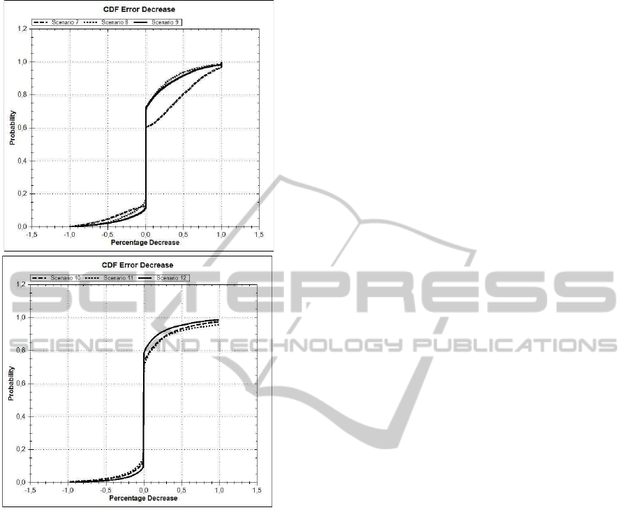
Figure 4: CDF’s of the relative forecast error reduction of
scenario seven to twelve.
shown that this detection problem can be solved by
adequate transformation routines that reflect changes
of interest. The special aim will be to design those
transformation routines with respect to efficiency and
robustness. Section 2.4 provided a brief note to this
topic in order to show the flexibility of the novel ap-
proach.
From the theoretical point of view the current ap-
plication is an offline detection problem. In future
work this algorithm will be applied to online detec-
tion problems, which demands new performance in-
dicators such as mean time between false alarms or
mean delay for detections.
The goal of this paper is to demonstrate the appli-
cability of the algorithm to a real-world problem and
facing real-world data. Future prospects will be to
analyze more general performance indicators as pro-
posed for example in (Basseville and Nikiforov,1993)
such as mean time between false alarms, probability
of false detections, mean delay for detection, proba-
bility of nondetection, statistical power, and required
effect size to name but a few. The goal will be to an-
swer these questions analytically and by simulation.
REFERENCES
Basseville, M. and Nikiforov, I. (1993). Detection of Abrupt
Changes: Theory and Application. Prentice-Hall,Inc.
Brown, R. (1959). Statistical forecasting for inventory con-
trol. McGraw-Hill New York.
Chandola, V., Banerjee, A., and Kumar, V. (2009).
Anomaly detection: A survey. ACM Computing Sur-
veys (CSUR), 41(3):1–58.
Chernoff, H. (1952). A Measure of Asymptotic Efficiency
for Tests of a Hypothesis Based on the Sum of Ob-
servations. The Annals of Mathematical Statistics,
23:493–507.
Feller, S., Chevalier, R., and Morsili, S. (2010). Parame-
ter Disaggregation for High Dimensional Time Series
Data on the Example of a Gas Turbine. In Proceedings
of the 38th ESReDA Seminar, Pcs, H, pages 13–26.
Feller, W. (2009). An introduction to probability theory and
its applications. Wiley-India.
Fujimaki, R., Yairi, T., and Machida, K. (2005). An
Approach to Spacecraft Anomaly Detection Prob-
lem Using Kernel Feature Space. In Proceedings of
the 11th ACM SIGKDD International Conference on
Knowledge Discovery in Data Mining, pages 401–
410. ACM.
Gardner Jr, E. (1985). Exponential smoothing: The state of
the art. Journal of Forecasting, 4(1):1–28.
Gelper, S., Fried, R., and Croux, C. (2010). Robust fore-
casting with exponential and Holt-Winters smoothing.
Journal of Forecasting, 29(3):285–300.
Guralnik, V. and Srivastava, J. (1999). Event Detection
from Time Series Data. In Proceedings of the 5th
ACM SIGKDD International Conference on Knowl-
edge Discovery and Data Mining, pages 33–42. ACM.
Gustafsson, F. (1998). Estimation and Change Detection
of Tire-Road Friction Using the Wheel Slip. IEEE
Control System Magazine, 18(4):42–49.
Hartigan, J. and Wong, M. (1979). Algorithm AS 136:
A k-means Clustering Algorithm. Journal of the
Royal Statistical Society. Series C (Applied Statistics),
28(1):100–108.
Holt, C. (1957). Forecasting trends and seasonals by expo-
nentially weighted moving averages. ONR Memoran-
dum, 52:1957.
Ibaida, A., Khalil, I., and Sufi, F. (2010). Cardiac abnor-
malities detection from compressed ECG in wireless
telemonitoring using principal components analysis
(PCA). In Intelligent Sensors, Sensor Networks and
Information Processing (ISSNIP), 2009 5th Interna-
tional Conference on, pages 207–212. IEEE.
ICINCO 2011 - 8th International Conference on Informatics in Control, Automation and Robotics
270

Ide, T. and Kashima, H. (2004). Eigenspace-based
Anomaly Detection in Computer Systems. In Pro-
ceedings of the 10th ACM SIGKDD International
Conference on Knowledge Discovery and Data Min-
ing, pages 440–449. ACM.
Kawahara, Y. and Sugiyama, M. (2009). Change-point De-
tection in Time Series Data by Direct Density-Ratio
Estimation. In Proceedings of 2009 SIAM Interna-
tional Conference on Data Mining (SDM2009), pages
389–400.
Ma, J. and Perkins, S. (2003). Time Series Novelty De-
tection Using One-class Support Vector Machines. In
Proceedings of the International Joint Conference on
Neural Networks, volume 3, pages 1741–1745.
Markou, M. and Singh, S. (2003). Novelty Detection: a
Review–Part 1: Statistical Approaches. Signal Pro-
cessing, 83(12):2481–2497.
Murad, U. and Pinkas, G. (1999). Unsupervised Profil-
ing for Identifying Superimposed Fraud. Principles
of Data Mining and Knowledge Discovery, 1704:251–
261.
Ng, T., Skitmore, M., and Wong, K. (2008). Using genetic
algorithms and linear regression analysis for private
housing demand forecast. Building and Environment,
43(6):1171–1184.
Pauli, D., Timm, I., Lorion, Y., and Feller, S. (2011). Using
Chernoff’s Bounding Method for High-Performance
Structural Break Detection. Submitted for publication.
Perron, P. (2006). Dealing with Structural Breaks. Palgrave
handbook of econometrics, 1:278–352.
Pinson, P., Nielsen, H., Madsen, H., and Nielsen, T. (2008).
Local linear regression with adaptive orthogonal fit-
ting for the wind power application. Statistics and
Computing, 18(1):59–71.
Press, W., Teukolsky, S., Vetterling, W., and Flannery, B.
(2007). Numerical Recipes: The Art of Scientific Com-
puting. Cambridge University Press.
Schwabacher, M., Oza, N., and Matthews, B. (2007).
Unsupervised Anomaly Detection for Liquid-Fueled
Rocket Propulsion Health Monitoring. In Proceedings
of the AIAA Infotech@ Aerospace Conference, Reston,
VA: American Institute for Aeronautics and Astronau-
tics, Inc.
Strang, G. (1989). Wavelets and dilation equations: A brief
introduction. Siam Review, 31(4):614–627.
Taylor, J. (2010). Multi-item sales forecasting with total
and split exponential smoothing. Journal of the Oper-
ational Research Society.
Wadsworth, H. (1997). Handbook of statistical methods for
engineers and scientists. McGraw-Hill Professional.
Xia, B. and Zhao, C. (2009). The Application of Multiple
Regression Analysis Forecast in Economical Forecast:
The Demand Forecast of Our Country Industry Lava-
tion Machinery in the Year of 2008 and 2009. In Sec-
ond International Workshop on Knowledge Discovery
and Data Mining, 2009. WKDD 2009, pages 405–408.
FORECAST ERROR REDUCTION BY PREPROCESSED HIGH-PERFORMANCE STRUCTURAL BREAK
DETECTION
271
