
ESTIMATION-DECODING ON LDPC-BASED 2D-BARCODES
W. Proß
1
, M. Otesteanu
1
and F. Quint
2
1
Faculty of Electronics and Telecommunications, Politehnica University of Timisoara, Timisoara, Romania
2
Faculty of Electrical Engineering and Information Technology, University of Applied Sciences, Karlsruhe, Germany
Keywords:
2D-Barcode, LDPC Code, Estimation-Decoding, Hidden-Markov-Model.
Abstract:
In this paper we propose an extension of the Estimation-Decoding algorithm for the decoding of our Data
Matrix Code (DMC), which is based on Low-Density-Parity-Check (LDPC) codes and is designed for use in
industrial environment. To include possible damages in the channel-model, a Markov-modulated Gaussian
channel (MMGC) was chosen to represent everything in between the embossing of a LDPC-based DMC and
the camera-based acquisition. The MMGC is based on a Hidden-Markov-Model (HMM) that turns into a two-
dimensional model when used in the context of DMCs. The proposed ED2D-algorithm (Estimation-Decoding
in two dimensions) is implemented to operate on a 2D-LDPC-Markov factor graph that comprises of a LDPC
code’s Tanner-graph and a 2D-HMM. For a subsequent comparison between different barcodes in industrial
environment, a simulation of typical damages has been implemented. Tests showed a superior decoding be-
havior of our LDPC-based DMC decoded with the ED2D-decoder over the standard Reed-Solomon-based
DMC.
1 INTRODUCTION
In 1952 the first barcode system was patented by J.
N. Woodland and B. Silver (Woodland and Silver,
1949). Today one dimensional barcodes are more and
more replaced by their two dimensional (2D) succes-
sors. They offer a high information-density as well
as an integrated error-correction capability in most
cases. One of the most successful 2D-barcodes is
the Data Matrix Code (DMC) which is internationally
standardized in (ISO/IEC, 2000). A DMC is formed
by the three major components, as shown in Figure
1. The finder-pattern is comprised of the solid bor-
der and the broken border. The L-shaped solid bor-
der helps in locating the DMC whereas the alternating
pattern of the broken border allows to determine the
DMC’s size. The data region contains the encoded in-
formation. Thereby a binary one is represented by a
black squared module and a binary zero by a white
squared module. This is only true if the DMC is
printed black on a white surface. When used in in-
dustrial environment the codes get stamped, milled
and laser-etched on different kinds of material. Fur-
thermore there are different kinds of interferences that
may disturb the barcode. Thereby decoding is much
more challenging.
2 LDPC-BASED DMC
Considering the application in industrial environment,
a 2D-barcode based on Low-Density-Parity-Check
(LDPC) codes was developed. The outer appearance
of our barcode is similar to that of the DMC since
the finder-pattern that surrounds a DMC has been
adopted.
PEG-LDPC Codes: The information is encoded
in our barcode by use of a regular PEG-LDPC
code unlike the standard DMC that is based on
Reed-Solomon (RS) codes. The first introduction of
LDPC codes has already been in 1962 by Gallager
(Gallager, 1962). Since the rediscovery of LDPC
codes by MacKay and Neal in 1995 (MacKay
and Neal, 1995), many further developments have
been published, making LDPC codes a serious
competitor to RS codes and the more recent Turbo
codes for many fields of application. One important
contribution was the introduction of the Progressive-
Edge-Growth (PEG) construction of the LDPC codes
underlying Parity-Check-Matrix (Hu et al., 2005) that
made LDPC codes attractive for short block length
applications as well. A single LDPC codeword is
used to fill the data region of the DMC because it is
well known that the decoding performance of LDPC
codes increases with the codeword-length.
34
Proß W., Otesteanu M. and Quint F..
ESTIMATION-DECODING ON LDPC-BASED 2D-BARCODES.
DOI: 10.5220/0003457400340039
In Proceedings of the International Conference on Signal Processing and Multimedia Applications (SIGMAP-2011), pages 34-39
ISBN: 978-989-8425-72-0
Copyright
c
2011 SCITEPRESS (Science and Technology Publications, Lda.)

Complete
Solid Border
Data Region
Broken Border
Figure 1: Three major parts of a DMC.
Symbol-placement: The procedure of placing the
LDPC codeword’s symbols within the available grid
of the DMC’s data region is done with respect to typ-
ical interferences that may occur in industrial envi-
ronment. The probability that damages caused by
dirt, rust, scratches, unequal illumination etc. affect
a contiguous part of the DMC is very high. Con-
sidering this, the symbol-nodes connected to the same
check-node in the LDPC code’s Tanner graph (Tan-
ner, 1981) are placed as far as possible from each
other in the data region under the constraint of the
limited area occupied by the code. This way each
check-node is affected by the fewest possible number
of disturbed symbol-nodes. The placement procedure
is based on an optimization process and is explained
in detail in (Proßet al., 2010). As an example, Figure 2
depicts the symbol-placement of three symbol-nodes
connected to the same check-node.
Image-processing: For the localization of the DMC,
the already known standard procedures are applied.
In contrast to the RS code used by the original DMC,
the LDPC decoder uses soft-decisions (SDs) as an in-
put. For the computation of these SDs a correlation
coefficient r
i j
is calculated for each module in row i
and column j of the DMC as follows:
r
i j
=
∑
h
k=1
∑
v
l=1
(x
i j
kl
− ¯x
i j
)(y
kl
− ¯y)
√
∑
h
k=1
∑
v
l=1
(x
i j
kl
− ¯x
i j
)
2
∑
h
k=1
∑
v
l=1
(y
kl
− ¯y)
2
(1)
k and l are the indices for the h horizontal and v
vertical pixels in each module respectively. Consider-
ing one module in row i and column j of the DMC,
x
i j
kl
denotes one pixel in row k and column l of the
module. y
kl
stands for one pixel in the reference mod-
ule. The reference module is generated based on an
averaging of all modules that belong to the DMC’s
finder-pattern and represent a binary one. ¯y and ¯x
i j
are the means of all the pixels referring to the refer-
ence module and the module in row i and column j of
the DMC, respectively.
3 DESIGN OF THE DECODER
The choice of an appropriate channel-model is es-
sential for the decoding success of the new designed
s
Tanner-
graph
s
s
!
s
"
#
= $
+ $
!
+ $
s
s
!
s
LDPC-based DMC
Figure 2: Symbol placement.
LDPC-based DMC. The channel-model has a high
impact on:
1. The design of the employed LDPC code;
2. The computation of the SDs passed to the LDPC
decoder;
3. The decoding procedure.
Therefore one has to study the DMC environment and
carefully choose an appropriate channel-model to rep-
resent everything in between the embossing and the
capturing of a DMC.
3.1 Channel-model in Absence of
Damages
In order to describe the distribution of the correlation-
coefficients computed by equation (1), one has to
find an appropriate channel-model. The correlation-
coefficients are separated into two data-sets referring
to one-modules and zero-modules respectively. Then
one has to choose a Probability-Density-Function
(PDF) for each of the two data-sets that together de-
scribe the channel.
The distribution is mainly affected by the
embossing-technique, the material and the camera-
based system. Thus various pictures of DMCs milled
on different types of material like aluminum, copper,
steel, brass and different colored plastic have been
analyzed. Thereby several cutting depths have been
considered as well. Dependent on the material, the
acquisition of the codes was done in a bright or a dark
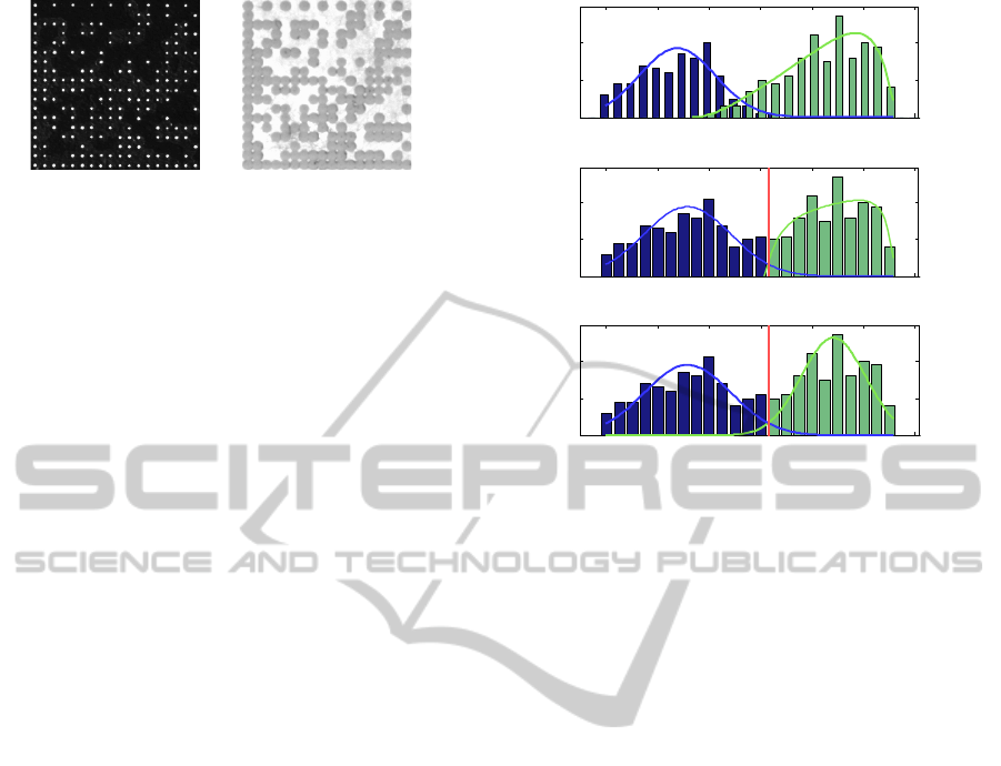
field. This can be seen in the two examples in Fig-
ure 3. In Figure 3(a) the DMC was milled on a plate
of steel and the illumination setting caused the cavi-
ties to reflect the light directly into the camera’s lens.
Opposed to that the surface reflects the light into the
camera in Figure 3(b) where the DMC was milled into
a white plate of plastic.
The test of the null hypotheses that the one-
samples and the zero-samples belong to a Gaussian
distribution was done based on a 5% Shapiro-Wilk
(SW) test as well as a 5% Anderson-Darling (AD)
test. Only in a few cases the null hypotheses have
not been rejected. Furthermore this was only true for
ESTIMATION-DECODING ON LDPC-BASED 2D-BARCODES
35
(a) Dark field (b) Bright field
Figure 3: DMC milled on a) steel b) white plastic.
the zero-modules. Because of that, another analysis
was done by use of the Johnson distribution (Johnson,
1949) (Johnson et al., 1994) that provides a system
of curves with the flexibility of covering a wide vari-
ety of shapes. Although the fitting to lots of different
shaped samples works very good, the Gaussian ap-
proximation was chosen in the context of DMCs. The
reason for that is explained using the example of Fig-
ure 3(b) and the corresponding histograms shown in
Figure 4. Figure 4(a) shows the histogram of the zero-
modules and the one-modules of the DMC under the
situation of correct labeling of the modules. Accord-
ing to the employed SW-test and the AD-test the zero-
modules belong to a Gaussian-distribution whereas
the hypothesis for a Gaussian distribution of the one-
modules has been rejected. Thus the histogram of the
zero-modules on the left side in Figure 4(b) has been
approximated by a Gaussian curve whereas the curve
on the right side stems from a Johnson fitting to the
histogram of the one-modules. It is well seen that the
two histograms as well as their fitted curves overlap
each other.
In contrast to the above, the codeword is
not known when considering a common decoding-
process of a DMC. For the purpose of estimating the
PDF of the two types of modules we provisionally
separate the modules into two classes by applying a
threshold to the correlation coefficients. The only dif-
ference between Figure 4(b) and Figure 4(c) is that
the fitting curve to the histogram of the one-modules
in Figure 4(b) is obtained by a Johnson fitting whereas
the approximation in Figure 4(c) has been done by us-
ing a Gaussian fitting. The zero-samples have been
approximated by a Gaussian-PDF in both cases as
the hypothesis-test has been successful. As seen in
Figure 4(b), the approximation of the histogram with
the Johnson PDF leads to an overfitting. This sug-
gest a good confidence for correlation values just be-
low the tentative threshold to belong to zero-modules.
In reality, this is not the case since the histograms of
the two classes heavily overlap. The suggested high
confidence leads to large log-likelihood ratios (LLRs)
which are used in the subsequent decoding algorithm.
In this case the advantage of soft-decoding is lost.
Furthermore, when calculating the LLRs based on a
−0.4 −0.2 0 0.2 0.4 0.6 0.8
0
10
20
(a) Real distribution
−0.4 −0.2 0 0.2 0.4 0.6 0.8
0
10
20
(b) Fitted with Gauss & Johnson
−0.4 −0.2 0 0.2 0.4 0.6 0.8
0
10
20
(c) Fitted with Gauss only
Figure 4: Histograms of correlation-coefficients separated
into one-modules and zero-modules.
Gaussian approximation, the histogram-skewness that
in many cases is responsible for the failure of the hy-
pothesis test, does not have a critical effect.
3.2 Channel-model for Damaged DMCs
The situation changes a lot when taking possible
damages into account. In industrial environment,
these are typically blots, scratches, dirt and rust as
well as effects caused by unequal illumination or
soiled camera-lenses. This leads to a change of the
gray-value distributions. In most cases one can ob-
serve a stretching of the histograms that refer to ones
and zeros respectively. Because of that a two-state
Markov-channel is utilized that includes possible ef-
fects caused by damages. The resulting channel-
model can be seen in Figure 5. The two states of the
Hidden-Markov Model (HMM) represent the follow-
ing two sub-channels:
Good Channel: This sub-channel is an Additive
White Gaussian Noise (AWGN) channel as described
in Section 3.1. This channel does not consider the
above mentioned damages and thus is referred to as
good channel.
Bad Channel: The second sub-channel is denoted as
bad channel and takes damages into account. It turns
out to be an AWGN channel as well, but with larger
variances compared to the good channel.
Thus the whole model represents a channel with
memory whose behavior is dependent on the current
underlying channel state. Moreover it is a Markov-
modulated Gaussian channel (MMGC) since it can be
SIGMAP 2011 - International Conference on Signal Processing and Multimedia Applications
36

−
Good
Channel
Bad
Channel
−
!!
!!
Figure 5: Channel-model based on a two-state hidden-
markov model.
16 vertical Markov-Chains
16
vertical Markov
-
Chains
16 horizontal Markov-Chains
16 horizontal Markov
-
Chains
Figure 6: Two-dimensional HMM.
described as a memoryless AWGN channel parame-
terized by the noise variances. The probabilities for
a transition from the good to the bad sub-channel and
vice versa are denoted as P
bad
and P
good
respectively.
3.3 ED2D-algorithm
The random-like connection of symbol-nodes with
check-nodes in a LDPC-code’s Tanner graph can
be interpreted as a build in interleaver. In tradi-
tional approaches channel interleavers are used to
obtain a channel which is assumed to be memory-
less. However, it has been shown (Wadayama, 2000)
(Garcia-Frias, 2004) (Ratzer, 2002) (Eckford, 2004)
that significant improvement is obtained by use of an
Estimation-Decoding (ED) algorithm that takes the
channel’s memory into account.
The ED-algorithm is based on the so called
Markov-LDPC factor graph which comprises two
subgraphs, namely the LDPC code’s Tanner-graph
and the Markov chain. On the Markov-subgraph a
state-estimation is computed by use of the Forward-
Backward algorithm that is similar to the BCJR-
algorithm (Bahl et al., 1974). This algorithm is
bit-wise connected with the Belief-Propagation -
algorithm (BPA) (Gallager, 1962) on the LDPC-
subgraph to form the ED-algorithm. So far ED of
LDPC codes has only been applied to time dependent
and thus one-dimensional systems.
Considering the application of Estimation-
Decoding on DMCs the one-dimensional timescale
turns into a geometry of two dimensions. This leads
to a replacement of one Markov-chain by several
Markov-chains. In our Estimation-Decoding in two
dimensions (ED2D), we assign a sub-Markov-chain
to each row and each column of the DMC’s data
region as depicted in the example in Figure 6. This
way the state-estimation referring to a single module
is based on a horizontal Markov-chain and a vertical
Markov-chain. The complete 2D-Markov-LDPC
factor graph that the ED2D-algorithm is based on
is depicted in Figure 7 and the messages of one
sector are shown in Figure 8. For clarity purposes
only the messages for the horizontal Markov-chain
are depicted. r and c are the indices for the rows
and columns of the 2D-Markov-subgraph. The
check-nodes
c
and the symbol-nodes
x
are part of
the LDPC-subgraph whereas the state-nodes s and
the channel-nodes (black squares) belong to the
Markov-subgraph. The soft-decisions (SDs), that the
ED2D-algorithm receives from our image-processing
part (Section 2) are denoted by y. The noise added
to the binary value of a DMC-module in row r and
column c is assumed to stem either from the good
sub-channel or the bad sub-channel of the MMGC
which is dependent on the state that the state-node s
r,c
is estimated to be in. S = {G, B} is the set of states
a state-node s
r,c
can be in, where G and B represent
the good and the bad sub-channel respectively. The
forward and backward messages are represented
by α and β respectively. The channel-message ζ is
send from the 2D-Markov-subgraph to the LDPC-
subgraph. χ is the extrinsic information passed from
the LPDC-subgraph to the 2D-Markov-subgraph.
The messages of the 2D-Markov-subgraph are
computed as follows.
Forward-message α:
α
h
r,c+1
(s
r,c+1
) =
∑
s
r,c
∈S
Pr(s
r,c+1
| s
r,c
)α
h
r,c
(s
r,c
)
·
∑
x
r,c
∈{0,1}
Pr(x
r,c
| χ
r,c
)Pr(y
r,c
| x
r,c
, s
r,c
)
(2)
Backward-message β:
β
h
r,c
(s
r,c
) =
∑
s
r,c+1
∈S
Pr(s
r,c+1
| s
r,c
)β
h
r,c+1
(s
r,c+1
)
·
∑
x
r,c
∈{0,1}
Pr(x
r,c
| χ
r,c
)Pr(y
r,c
| x
r,c
, s
r,c
)
(3)
where Pr(s
r,c+1
| s
r,c
) is one of the four transition
probabilities of Figure 5. The computation of the
messages α
v
and β
v
for the vertical Markov-chains of
Figure 6 are likewise. The channel-message ζ passed
to the LDPC-subgraph is computed based on the mes-
ESTIMATION-DECODING ON LDPC-BASED 2D-BARCODES
37

Figure 7: 2D-Markov-LDPC factor graph.
sages α
h
and β
h
of the horizontal Markov-Chain and
the messages α
v
and β
v
of the vertical Markov-Chain:
ζ
r,c
=log
Pr(x
r,c
= 0 | α
h
r,c
(s
r,c
)β
h
r,c+1
(s
r,c+1
))
Pr(x
r,c
= 1 | α
h
r,c
(s
r,c
)β
h
r,c+1
(s
r,c+1
))
+log
Pr(x
r,c
= 0 | α
v
r,c
(s
r,c
)β
v
r+1,c
(s
r+1,c
))
Pr(x
r,c
= 1 | α
v
r,c
(s
r,c
)β
v
r+1,c
(s
r+1,c
))
(4)
with
Pr(x
r,c
= 0 | α
h
r,c
(s
r,c
), β
h
r,c+1
(s
r,c+1
)) =
∑
s
r,c
∈S
∑
s
r,c+1
∈S
Pr(y
r,c
| x
r,c
= 0, s
r,c
)
· Pr(s
r,c+1
| s
r,c
)α
h
r,c
(s
r,c
)β
h
r,c+1
(s
r,c+1
)
(5)
h and v refer to horizontal and vertical rows respec-
tively. Concerning the application of the ED2D-
algorithm in the context of DMCs, the DMC’s finder-
pattern offers another advantage next to the original
purpose. Since the values of the finder-pattern are al-
ways known, the corresponding messages χ do not
change during the iterative ED2D-decoding so that
Pr(x
r,c
| χ
r,c
) =
{
0 , x
r,c
= 0
1 , x
r,c
= 1
∀x
r,c
∈ F
1
(6a)
and
Pr(x
r,c
| χ
r,c
) =
{
1 , x
r,c
= 0
0 , x
r,c
= 1
∀x
r,c
∈ F
0
(6b)
with F
1
={one-modules of the finder-pattern} and
F
0
={zero-modules of the finder-pattern}. The
channel-message ζ and the extrinsic message χ re-
present the interface from the 2D-Markov-subgraph
to the LDPC codes Tanner-graph on which the mes-
sages are computed based on a common BPA (Gal-
lager, 1962).
,
!
,
"
,
"
,#$
%
,
&
,
&
,#$
'
,#$
'
,
(
,
)
,
*
,
(
LDPC –
subgraph
Markov –
subgraph
Horizontal
Markov-Chain
Figure 8: Local messages in the 2D-Markov-LDPC factor
graph.
4 IMPLEMENTATION & TEST
The ED2D-algorithm has been tested based on a
DMC of size 26 × 26. The data has been encoded
with a rate 0.61 regular PEG-LDPC code of length
n = 576. The finder-pattern that surrounds the 24 ×24
size data region and the code rate referring to the
DMC size have been chosen conforming to standard
(ISO/IEC, 2000). The 576 bits of the LDPC codeword
have been placed in the data region using the opti-
mization technique described in (Proßet al., 2010).
For comparison purposes the new designed
LDPC-based DMC and the original RS-based version
have been milled one next to the other on three differ-
ent kinds of material. For both versions, the informa-
tion to be encoded, the DMC-size and the code rate
have been chosen identically. In addition, the condi-
tions of the following acquisition and image process-
ing were exactly the same for all DMC-pairs. To in-
clude possible damages, a simulation of water drops
and oil drops was integrated. The simulation en-
sured that both versions of the DMC were interfered
with identical damages. An example of the damage-
simulation can be seen in Figure 9. For this test plates
of brass, aluminum and grey plastic have been used.
Each DMC was interfered with 10 simulated versions
of oil drops and water drops respectively. Thus, for
each material there have been two DMC versions pair-
wise interfered with 20 different disturbances. All in
all 60 interfered LDPC-based DMCs were compared
with 60 RS-based DMCs affected by exactly the same
damages.
The test results are shown in Figure 10. Success-
ful decodings are counted according to the material
and the type of damages. The last line shows the cu-
mulative percentage of succeeded decodings. With a
success rate of 92% our LDPC-based DMC decoded
with the ED2D-decoder clearly outperforms the stan-
dard DMC of which only 53% succeeded in decoding.
SIGMAP 2011 - International Conference on Signal Processing and Multimedia Applications
38
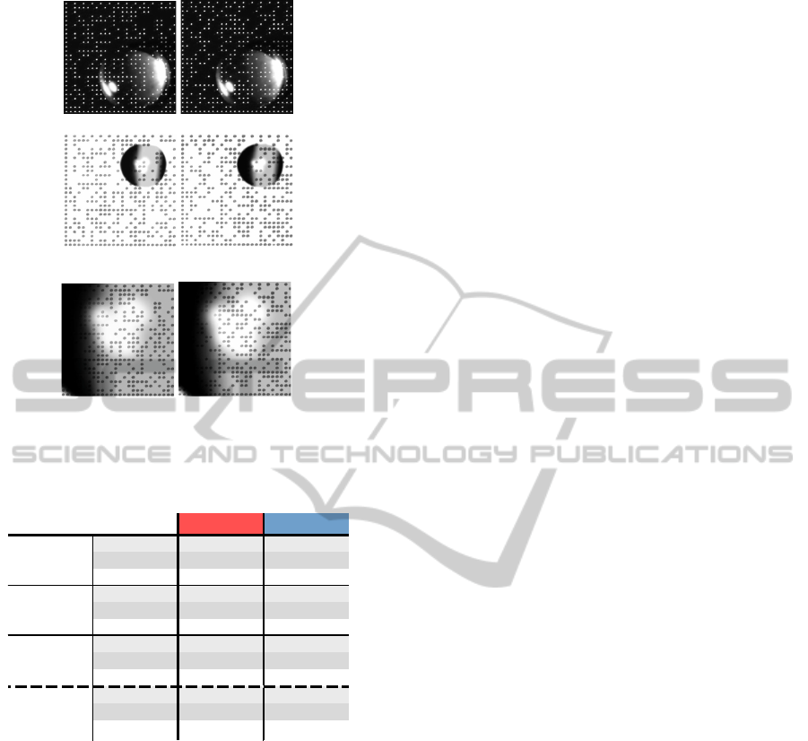
(a) LDPC DMC (b) Original DMC
(c) LDPC DMC (d) original DMC
(e) LDPC DMC (f) original DMC
Figure 9: DMC-pairs milled on the same plate of brass
and interfered with simulated water drop (a and b) and alu-
minum and interfered with simulated oil drop of size larger
than the DMC (c, d, e and f).
ED2D RS
water 9 4
oil 8 4
total 17 8
water 10 7
oil 10 10
total 20 17
water 10 4
oil 8 3
total 18 7
water 97% 50%
oil 87% 57%
Total 92% 53%
Plastic
Total
Successfully decoded
Aluminum
Brass
Figure 10: comparison results of 60 tests.
5 CONCLUSIONS
For the decoding of LDPC-based DMCs an algo-
rithm called ED2D-algorithm was established. This
decoding-algorithm is an extension of the one-
dimensional ED-algorithm. ED2D-decoding is based
on a two-dimensional Hidden-Markov-Model that has
been constructed in order to include possible dam-
ages into the underlying channel-model. Two types
of damages that are typical in industrial environment
were simulated. Based on the damage-simulation
a testing showed a superior decoding behavior of
our LDPC-based DMCs decoded with the ED2D-
algorithm compared to the standard RS-based DMC.
ACKNOWLEDGEMENTS
This work is part of the project MERSES and has been
supported by the European Union through its Euro-
pean regional development fund(ERDF) and by the
German state Baden-W
¨
urttemberg. We would like to
thank the reviewers for helpful comments.
REFERENCES
Bahl, L. R., Cocke, J., Jelinek, F., and Raviv, J. (1974). Op-
timal decoding of linear codes for minimizing symbol
error rate. IEEE Transactions on Information Theory,
20(2):284–287.
Eckford, A. W. (2004). Low-density parity-check codes for
Gilbert-Elliott and Markov-modulated channels. PhD
thesis, University of Toronto.
Gallager, R. G. (1962). Low density parity check codes.
IRE Transactions on Information Theory, 1:21–28.
Garcia-Frias, J. (2004). Decoding of low-density parity-
check codes over finite-state binary markov channels.
IEEE Transactions on Communications, 52(11):1841.
Hu, X. Y., Eleftheriou, E., and Arnold, D. M. (2005).
Regular and irregular progressive edge-growth tanner
graphs. IEEE Transactions on Information Theory,
51(1):386–398.
ISO/IEC (2000). 16022:2000(e) information technology —
international symbology specification — data matrix.
Johnson, N. L. (1949). Systems of frequency curves gen-
erated by methods of translation. Biometrika,36(1-
2):149.
Johnson, N. L., Kotz, S., and Balakrishnan, N. (1994). Con-
tinuous univariate distributions. A Wiley-Interscience
publication. Wiley, New York, 2. ed. edition.
MacKay, D. and Neal, R. (1995). Good codes based on very
sparse matrices. Cryptography and Coding, pages
100–111.
Proß, W., Quint, F., and Otesteanu, M. (2010). Using peg-
ldpc codes for object identification. In Electronics and
Telecommunications (ISETC), 2010 9
th
, pages 361-
364.
Ratzer, E. A., editor (2002). Low-density parity-check codes
on Markov channels, Proceedings of 2nd IMA Con-
ference on Mathematics and Communications, Lan-
caster, U.K.
Tanner, R. M. (1981). A recursive approach to low com-
plexity codes. IEEE Transactions on Information The-
ory, 27:533–547.
Wadayama, T., editor (2000). An iterative decoding algo-
rithm of low density parity check codes for hidden
Markov noise channels, Proceedings of International
Symposium on Information Theory and Its Applica-
tions, Honolulu, Hawaii, USA.
Woodland, J. N. and Silver, B. (1949). U.S. Patent No.
2,612,994. Washington, DC: U.S. Patent and Trade-
mark Office.
ESTIMATION-DECODING ON LDPC-BASED 2D-BARCODES
39
