
STUDY OF THE PHENOMENOLOGY OF DDOS NETWORK
ATTACKS IN PHASE SPACE
Michael E. Farmer and William Arthur
Department of Computer Science, Engineering and Physics, University of Michigan-Flint, 303 E. Kearsley St., Flint, U.S.A.
Keywords: Denial of service, Computer networks, Computer viruses, Chaos.
Abstract: Denial of Service (DOS) network attacks continue to be a widespread problem throughout the internet.
These attacks are designed not to steal data but to prevent regular users from accessing the systems. One
particularly difficult attack type to detect is the distributed denial of service attack where the attacker
commandeers multiple machines without the users’ awareness and coordinates an attack using all of these
machines. While the attacker may use many machines, it is believed that the underlying characteristics of
the resultant network traffic are fundamentally different than normal traffic due to the fact that the
underlying dynamics of sources of the data are different than for normal traffic. Chaos theory has been
growing in popularity as a means for analyzing systems with complex dynamics in a host of applications.
One key tool for detecting chaos in a signal is analyzing the trajectory of a system’s dynamics in phase
space. Chaotic systems have significantly different trajectories than non-chaotic systems where the
trajectory of the chaotic system tends to have high fractal dimension due to its space filling nature, while
non-chaotic systems have trajectories with much lower fractal dimensions. We investigate the fractal nature
of network traffic in phase space and verify that indeed traffic from coordinated attacks have significantly
lower fractal dimensions in phase space. We also show that tracking the signals in either number of ports or
number of addresses provides superior detectability over tracking the number of bytes.
1 INTRODUCTION
Denial of Service (DOS) network attacks continue to
be widespread throughout the internet.
Consequently, considerable research has been
focused on developing algorithms for detecting DOS
and distributed DOS attacks based on the
characteristics of the incoming data patterns (Li,
2006); (Li, 2006); (Xiang et al., 2004);
(Limwiwatkul and Rungsawang, 2004); (Mitrokotsa
and Douligeris, 2005); (Oke et al., 2007); (Loukas
and Oke, 2007). The first step to developing a
successful detection algorithm is to determine the
characteristics of the data which may support the
discrimination of attacks from traditional traffic.
There are a variety of available standard datasets,
however, the authors have found these data sets have
one of three limitations: (i) they are from ‘honey
pot’ servers where limited normal traffic and attack
data are available, (ii) they are semi-fabricated
where simulated attack data is added to normal
traffic, or (iii) the entire data set is simulated, where
these datasets include MIT, DARPA, USC,
Berkeley, and KDD datasets (Li, 2006); (Mitrokotsa
and Douligeris, 2005); (Oke et al., 2007). The
current research discussed in this paper is unique in
that it is developed around actual network traffic
from the main server within the University of
Michigan-Flint Information Technology Services
(ITS) system. Hence the data represents significant
portions of real-world traffic collected in two
independent collection exercises three months apart
in time. These data sets contain actual orchestrated
known attacks from the parent school’s (University
of Michigan in Ann Arbor) ITS organization which
regularly tests the three campuses of the university
system for security weaknesses, including using
DOS and DDOS attacks.
By their very nature, DDOS attacks are designed
to be hidden from the network routers until the point
where they overwhelm the systems. Korn and Faure
(2003) note that ‘the tools of nonlinear dynamics
have become irreplaceable for revealing hidden
mechanisms”. Specifically, chaos theory has been
successfully used to model many naturally occurring
processes in physics, and most recently have also
78
E. Farmer M. and Arthur W..
STUDY OF THE PHENOMENOLOGY OF DDOS NETWORK ATTACKS IN PHASE SPACE.
DOI: 10.5220/0003460800780089
In Proceedings of the International Conference on Security and Cryptography (SECRYPT-2011), pages 78-89
ISBN: 978-989-8425-71-3
Copyright
c
2011 SCITEPRESS (Science and Technology Publications, Lda.)

found success in modeling biological neural activity
(Korn and Faure, 2003). In this paper, we are
motivated from research in chaos theory to analyze
the signals in phase space since as Tel and Gruiz
(2006) note “[one difference] between chaotic and
non-chaotic systems is that, in the former case, the
phase space objects … trace out complicated
(fractal) sets, whereas in the non-chaotic case the
objects suffer weak deformations”. Since it is
extremely difficult to prove the existence of chaos in
finite duration signals, Velaquez (2005) proposes a
more pragmatic approach by suggesting “attractor-
like” behavior of signals rather than committing to
the existence of true chaos. He also notes that the
non-predictable nature of [these] signals may be
neither from chaos or stochastic origins but from an
aperiodic forcing phenomenon.
In this paper we will demonstrate that both
normal network traffic and DOS network traffic
exhibit interesting yet dramatically different
trajectories in phase space, and that fractal analysis
of the phase space will provide a mechanism for
differentiating DDOS attacks from normal network
traffic in an actual university-wide network. The key
contributions of the research discussed in this paper
are: (i) propose analyzing network traffic in phase
space for detecting DDOS attacks, (ii) provide a
characterisation of normal network traffic versus
known DDOS attack traffic in phase space, (iii)
provide this characterization on actual real-world
data, collected from the main network of a
university, and (iv) use these characterizations to
identify the best network traffic data fields for
detecting DDOS attacks and provide values for the
key analysis parameters to analyze these signals.
2 RELATED WORK
There are a number of directions of algorithmic
approaches addressing DDOS detection, including:
neural networks operating on raw network data
(Mitrokotsa and Douligeris, 2005), second-order
statistical measures of traffic (Li et al., 2008);
(Rohani et al., 2007); (Feinstein et al., 2003) and
rule-based detection (Limwiwatkul and
Rungsawang, 2004).
There have also been a number of studies using
fractal-related measures of the time-domain network
signals to detect attacks, including measures based
on long-range dependencies using the Hurst
parameter (Li, 2006); (Xiang, Lin, Lei, and Huang,
2004), a hybrid approach using raw data and Hurst
parameters (Oke et al., 2007), and more recently
multi-fractal analysis (Liangxiu et al., 2002);
(Masugo, 2002). One team has even analyzed
network signals in phase space, however, it was for
the detection of worms rather than DDOS attacks Hu
et al., (2007). The directions of research using the
Hurst parameter and multi-fractal analysis are based
on the fact that network traffic is comprised of a
large number of individual connections with high
variability in duration and number of packets.
These various studies also used a variety of data
fields with which they analyzed the network traffic.
The most common data across these studies are the
number of bytes or the number of packets
transmitted within a time window with the following
researchers using either of these values exclusively
(Liangxiu et al., 2002); (Masugo, 2002); (Li, 2006);
(Xiang et al., 2004).
Researchers such as (Limwiwatkul and
Rungsawang, 2004); (Mitrokotsa and Douligeris,
2005); (Oke et al., 2007) recognized that more
sophisticated attacks, which exploit network security
weaknesses other than basic bandwidth limitations,
require the analysis of additional data fields such as:
- number of source IP addresses per time interval
- number of destination IP addresses per time
interval
- delay of packets within router
- number of source ports per time interval
- number of destination ports per time interval
- etc.
3 NETWORK TRAFFIC
PARAMETERS
Recognizing that DDOS attacks are becoming
increasingly sophisticated, in this study we will
analyze the phase space characteristics for normal
and DDOS attack signals for the following data
types:
- number of bytes,
- number of source and destination IP addresses, and
- number of source and destination ports.
For analyzing network data the instantaneous signal
has been shown to be not as important as the
aggregated signal within a time window (Masugo,
2002); (Li and Zhao, 2008); (Gregg et al., 2001);
(Li, 2006); (Piskozub, 2002). The aggregation
window is set in terms of milliseconds rather than
incoming data samples since we are specifically
interested in the temporal variations (i.e. bursts) in
the signal. Specifically for distributed DOS attacks
STUDY OF THE PHENOMENOLOGY OF DDOS NETWORK ATTACKS IN PHASE SPACE
79

we anticipate that the measures such as number of
source IP addresses and number of source ports per
time interval may be valuable measures. Also we
will demonstrate that for port and destination
address-based attacks, there is actually a very
interesting behavior of the aggregated number of
bytes per time interval during attacks.
4 FRACTAL MEASURES IN
PHASE SPACE
When analyzing a time series, the most common
measure for detecting chaos is the calculation of the
Lyapunov exponents (and all related measures) of
the phase space trajectories, which provide “ useful
bounds on the dimensions of the attractors”
(Eckmann and Ruelle, 1985). Eckmann and Ruelle
(1985) also state that: “the Lyapunov exponents, the
entropy, and the Hausdorff dimension associated
with a phase plot …all are related to how excited
and how chaotic a system is”. From the domain of
fractal analysis, there are three classes of measures
used for computing fractal dimensions: (i)
morphological dimensions, (i) entropy dimensions
and (iii) transform dimensions (Kinsner, 2005).
When applied to analyzing chaotic dynamics, these
morphological measures are applied to the phase
space plot to estimate the fractal dimension, where
higher fractal dimensions imply the existence of
chaos.
Most morphological-based dimension measures
are either directly related to or motivated by the
Hausdorff dimension,
A
s
h
which is defined as
(Peitgen, Jurgens, and
Saupe, 1992):
0
0
i
s
i
UdiaminflimA
s
h
,
(1)
where
i
U
is the set of hyperspheres of dimension s
and of diameter of
i
Udiam
, providing an open
cover over space A.
While the Hausdorff dimension is a member of
the morphological dimensions, it is not easily
calculated. Fortunately, there are numerous
dimensions, such as the Box Counting dimension
which are closely related (and provably upper
bounds to the Hausdorff dimension) and are
attractive because they are relatively easy to
compute (Kinsner, 2005). The Information
dimension is another closely related dimension
which is also quite popular and in some cases
believed to be more effective, but slightly more
complicated to compute compared to the Box
Counting method (Kinsner, 2005). The Box
Counting dimension
A
B
dim
is defined as (Peitgen
et al., 1992); (Theiler, 1990):
log
Nlog
limA
B
dim
A
0
,
(2)
where
AN
is the smallest number of boxes of size
that cover the space A. Very simply, the Box
Counting dimension is a computation of the number
of boxes of a given size within which some portion
of the trajectory can be found. Note, however, that it
does not count how many points from the trajectory
fall within the box. The Information dimension
provides a weight as to how often the trajectory can
be found in the box and is defined based on
Shannon’s definition of the sum of the information
across all boxes at a given resolution (Theiler,
1990); (Roberts, 2005):
i
i
P
i
PS ,
2
log
(3)
A
ii
BP
/ where
is the density of the phase plot
trajectory inside box B
i
and
A
is the overall
density of the entire trajectory. The Information
Dimension, f
info
, is then defined to be (Theiler,
1990):
log
0
lim
inf
S
Af
o
(4)
The management of the box sizes and their
overlay upon the phase plot are identical in each
method. A simple least squares fit of the log-log plot
of the number of boxes required for the cover versus
the box dimension provides the final dimensional
measure. For all of the analysis in this paper, the
Information dimension will be used since it is more
robust to low amplitude stray orbits in the
trajectories since it weights how often a particular
box is visited (Roberts, 2005).
5 PROCESSING TIME SERIES IN
PHASE SPACE
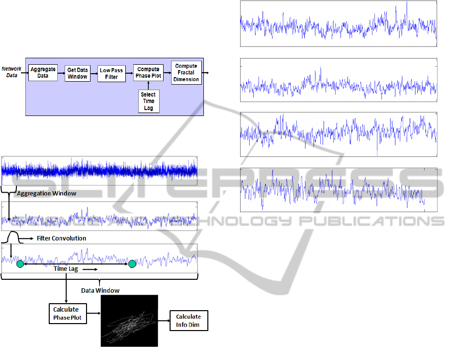
The processing flow for analyzing network traffic
data in phase space is provided in Figure 1. The
network traffic data we will be analyzing consists of
the packet header information collected using TCP-
Dump. The critical parameters which we will be
SECRYPT 2011 - International Conference on Security and Cryptography
80
analyzing to determine an optimal range of values
are: (i) Aggregation Window Length, (ii) Data
Window Length, (iii) Low Pass Filter Length, and
(iv) Time Lag, and a graphical representation of how
each fits into the data collection process is provided
in Figure 2. The first step in the processing is to
aggregate data.
Figure 1: Processing flow for phase space analysis of
network traffic.
Figure 2: Representation of the various critical data values
to be analyzed.
When we analyze normal network traffic packet
headers as shown in Figure 3 does not appear
significant as can be seen by the modest changes in
the phase plots shown in Figure 5, with a window
between 5 and 50 milliseconds providing roughly
the same fractal dimension (f
info
varies from 1.43 to
1.54 in this range). Likewise the varying time
domain behavior of an attack signal for a range of 5
to 50 milliseconds in Figure 4 and their
corresponding phase plots in Figure 6. The phase
plots provided in Figure 5 and Figure 6 show the
dramatic difference in the structure of the phase plot
for normal traffic versus attack traffic. The
difference in the structure of these phase plots
clearly reinforce the comments mentioned in the
introduction by Tel and Gruiz (2006) regarding the
relative complexity of phase plots between normal
and chaotic data. The analysis of this section of the
paper will determine the optimal parameters for
detecting and hence exploiting this difference.
(a)
(b)
(c)
(d)
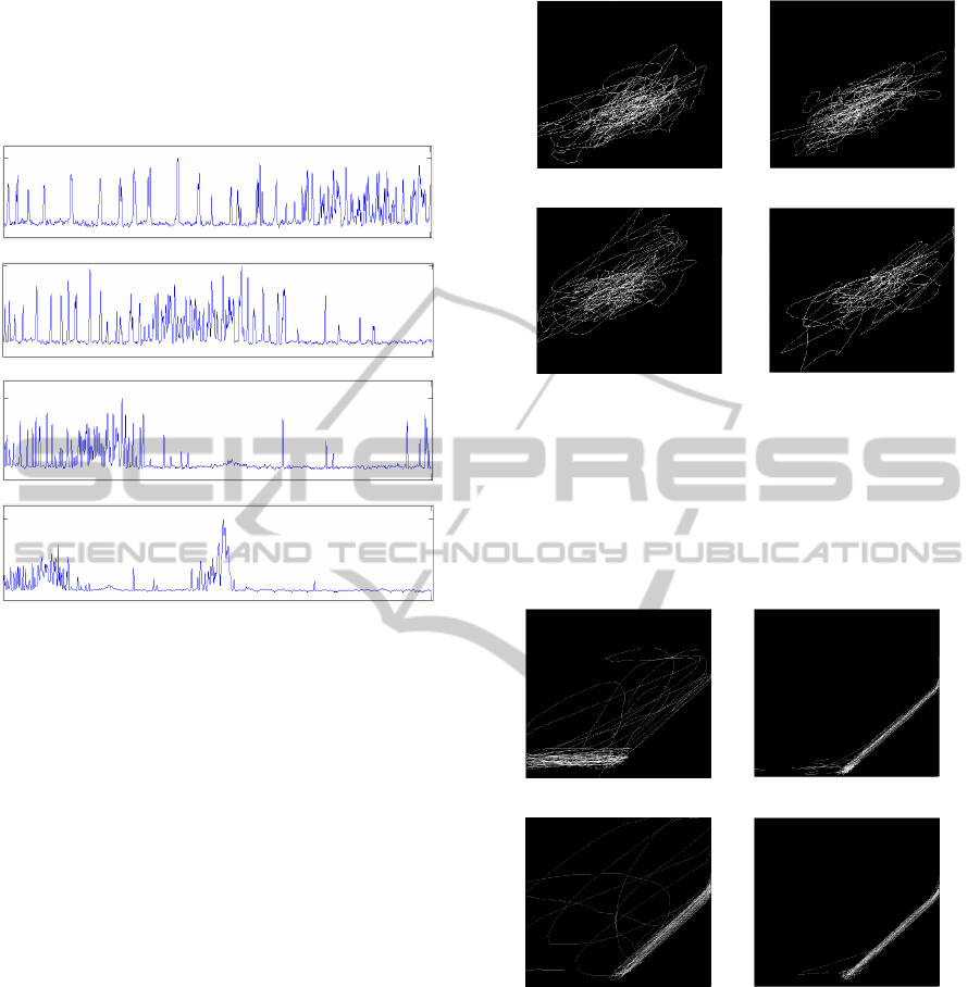
Figure 3: Time series for number of source ports for 7000
samples with 5000 point time lag for normal signal traffic:
(a) 5 millisecond aggregation window, (b) 10 millisecond
aggregation window, (c) 20 millisecond aggregation
window, and (d) 50 millisecond aggregation window.
One tradeoff on the aggregation window will be
the sheer magnitude of the data to be integrated. We
would like to eventually develop algorithms for
detecting and removing these chaotic signals within
the network routers and hence would like to
maintain reasonable data lengths. As we see in
Figure 4 aggregation windows as short as 5-10
milliseconds provide reasonable signal
manifestation. Another factor to maintain shorter
aggregation windows is that longer windows can
adversely affect the non-chaotic nature of an attack
signal since it will be buried in an extremely large
amount of normal network traffic. This effect can be
seen in Figure 7 showing the histograms of the
Information Dimension calculated for a run within a
data file containing known attack signals
interspersed in a background of normal traffic. Thus
there should be two peaks in the histogram, one
corresponding to the periods of attack and one
during periods of normal traffic. These histograms
were generated for 5, 10, 20, and 50 millisecond
aggregation windows. Notice at the longer 50
millisecond aggregations the attacks become masked
by the normal traffic and there is no clear distinction
in the histogram. Likewise there appears to be the
beginnings of a breakdown in separability at 20
STUDY OF THE PHENOMENOLOGY OF DDOS NETWORK ATTACKS IN PHASE SPACE
81
milliseconds, and the clearest distinction between
attack and normal traffic is at 10 milliseconds, where
the separability is actually quite promising. Thus for
the remainder of this study we will use a 10
millisecond aggregation period.
(a)
(b)
(c)
(d)
Figure 4: Time series for number of source ports for 7000
samples with 5000 point time lag for attack signal traffic:
(a) 5 millisecond aggregation window, (b) 10 millisecond
aggregation window, (c) 20 millisecond aggregation
window, and (d) 50 millisecond aggregation window.
The second step of the processing is to build the
data windows from which the phase plots will be
constructed. Its value is driven by the desired time
lag and number of points that can be used to build
the trajectories in phase space. Shorter times are not
representative, and longer times have less negative
impact but do increase processing and storage loads.
We found that between 1000 and 2000 samples
build a robust and representative phase space
trajectory. Note that the actual time duration of these
data windows will vary since we are integrating
numbers of aggregated samples rather than specific
time periods. We will show in subsequent analysis
that a 5000 point time lag produces the best
separation in fractal dimension between normal and
attack traffic. The combination of desired lag time
and adequacy of developed phase space trajectory
results in the selected time window to be 7000
samples.
Amplitude
Amplitude
Delta Amplitude Delta Amplitude
(a) (b)
Amplitude
Amplitude
Delta Amplitude Delta Amplitude
(c) (d)
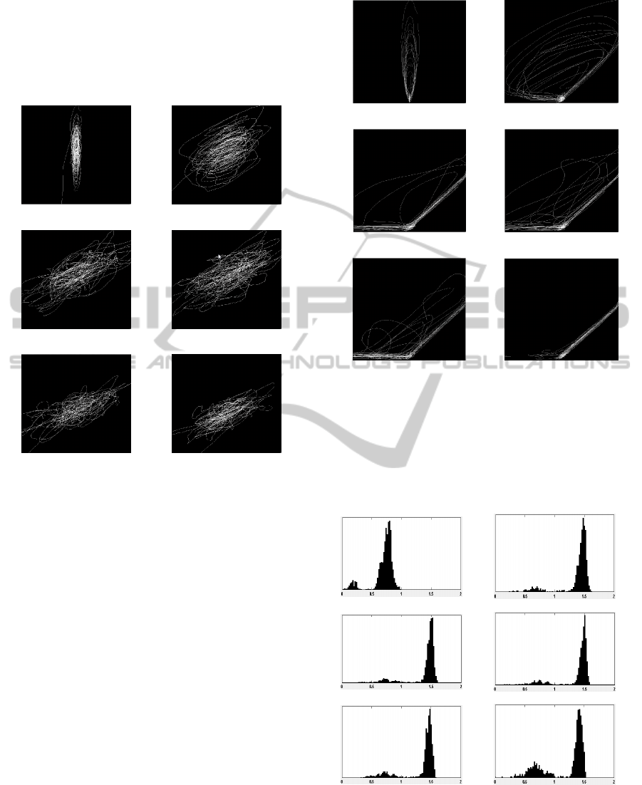
Figure 5: Exploring the effect of aggregation window size
on phase plot for number of source ports of 7000
aggregated samples with a time lag of 5000 for normal
traffic: (a) 5 millisecond aggregation window (f
info
=1.41),
(b) 10 millisecond aggregation window (f
info
=1.34), (c) 20
millisecond aggregation window (f
info
=1.35), and (d) 50
millisecond aggregation window (f
info
=1.31).
Amplitude
Amplitude
Delta Amplitude Delta Amplitude
(a) (b)
Amplitude
Amplitude
Delta Amplitude Delta Amplitude
(c) (d)
Figure 6: Exploring the effect of aggregation window size
on phase plot for number of source ports of 7000
aggregated samples with a time lag of 5000 for attack
traffic: (a) 5 millisecond aggregation window (f
info
=1.30),
(b) 10 millisecond aggregation window (f
info
=0.81), (c) 20
millisecond aggregation window (f
info
=0.99), and (d) 50
millisecond aggregation window (f
info
=0.74).
The third step in the processing defined in Figure
1 is to apply a low pass filter to the aggregated data
stream. Low pass filtering is a critical step in the
processing since it has been found that the presence
of noise can mask the effects of chaos in phase
SECRYPT 2011 - International Conference on Security and Cryptography
82
space, which is tellingly shown in the phase plots of
Figure 10 (a) and Figure 11 (b). The length of the
low-pass filter is a particularly sensitive parameter
since having too large of a filter window will
introduce correlation in the signal and likewise
distort the chaotic nature of the underlying signal,
thereby reducing the space-filling nature of the
trajectory (Rosenstein and Collins, 1994).
(a) (b)
(c) (d)
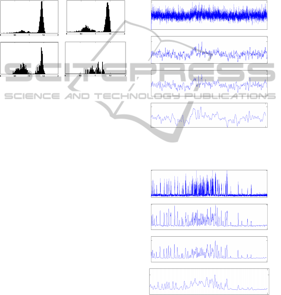
Figure 7: Histograms of the fractal dimensions calculated
with aggregation window size on phase plot for number of
source ports of 7000 aggregated samples with a time lag of
5000 for network traffic containing both normal traffic
(higher fractal dimensional peak) and attack traffic (lower
fractal dimensional peak): (a) 5 millisecond aggregation
window, (b) 10 millisecond aggregation window, (c) 20
millisecond aggregation window, and (d) 50 millisecond
aggregation window.
The signal characteristics for normal traffic of
the number of source ports ranging from raw data
(filter length of one) to a filter integration window of
50 samples is provided in Figure 8, and the resultant
phase plots of these signals are provided in Figure
10. Likewise signal characteristics for attack traffic
of the number of source ports ranging from raw data
(filter length of one) to a filter integration window of
50 samples is provided in Figure 9 and the resultant
phase plots of these signals are provided in Figure
11. In Figure 10 (a) the randomness of the phase plot
for normal traffic is due to the underlying noise,
while in Figure 10 (b) the structure of the phase plot
becomes apparent. Note how the trajectory of the
signal is less space filling from Figure 10 (b) and (c)
to Figure 10 (d) as the filter window increases to 50
samples. The noise in the signal is also clearly
visible in the phase plot of the attack signal without
filtering shown in Figure 11 (a). Also as the filter
length increases, the fact that the longer filter can
negatively impact the fractal nature of the
underlying signal can be witnessed clearly when
comparing Figure 12 (a) and (b) of the histograms
of the fractal dimension of the network traffic.
Notice that the large peak on the right side of the
histogram is clearly separable from the non-fractal
traffic represented by the lower fractal dimension
left peak in Figure 12 (a) while in Figure 12 (b) the
peak of higher fractal dimension has dramatically
migrated to the left hence mixing with the lower
fractal dimension peak thereby greatly reducing the
separability of the normal and attack traffic.
(a)
(b)
(c)
(d)
Figure 8: Time series for number of source ports for
normal signal traffic: (a) without filtering, (b) with 10
point low pass filter, (c) with 20 point low pass filter, and
(d) with 50 point low pass filter.
(a)
(b)
(c)
(d)
Figure 9: Time series for number of source ports for attack
signal traffic: (a) without filtering, (b) with 10 point low
pass filter, (c) with 20 point low pass filter, and (d) with
50 point low pass filter.
STUDY OF THE PHENOMENOLOGY OF DDOS NETWORK ATTACKS IN PHASE SPACE
83
A window size between ten and twenty samples
appears optimal for unmasking the underlying
trajectory structure and providing the greatest
separation in the fractal dimension of the normal and
attack traffic as can be seen from the fractal
dimension of Figure 10 (b) and Figure 11 (b). Since
the shorter window requires less processing we will
use a ten point Gaussian low-pass filter for all the
signals in this paper.
Amplitude
Amplitude
Delta Amplitude Delta Amplitude
(a) (b)
Amplitude
Amplitude
Delta Amplitude Delta Amplitude
(c) (d)
Figure 10: Exploring the effects of low pass filtering on
phase plot for number of source ports (7000 samples with
5000 point time lag) for normal signal traffic: (a) without
filtering (f
info
=1.20), (b) with 10 point low pass filter (f
info
=1.30), (c) with 20 point low pass filter (f
info
=1.32), and
(d) with 50 point low pass filter (f
info
=1.12).
The fourth stage in the processing defined in
Figure 1 performs the actual generation of the phase
plots. One key value we will see is also the Lag
Time which is critical to the construction of the
phase plots. The phase plot of the signal is computed
by mapping each point in the time series to an
(amplitude, delta amplitude) location. The delta
amplitude value is computed by comparing a
specific time series point i, with a sample i - ∆t,
where ∆t is referred to as the time lag. This sequence
of values calculated for each point in the time series
creates the trajectory in phase space. For time lags
that are too small, the chaotic nature of the signal
does not emerge, and the trajectory remains confined
to a smaller region of phase space as can be seen in
Figure 13 (a) and Figure 14 (a) for normal and attack
traffic respectively. As the time lag is increased, the
chaotic trajectory begins to emerge as is seen in
Figure 13 (b) and Figure 14 (b). To generate the
phase plots in Figure 13 and Figure 14 we needed to
maintain a constant length of the phase space
trajectory so while the aggregation value was fixed
at ten for each and the low pass filter length was
fixed at ten, the window lengths was varied so that
each trajectory consisted of 2000 points. Notice that
in for the normal traffic phase plots in Figure 13, the
fractal dimension is varies only slightly between f
info
= 1.3 and f
info
= 1.4.
Amplitude
Amplitude
Delta Amplitude Delta Amplitude
(a) (b)
Amplitude
Amplitude
Delta Amplitude Delta Amplitude
(c) (d)
Figure 11: Exploring the effects of low pass filtering on
phase plot for number of source ports (7000 samples with
5000 point time lag) for attack signal traffic: (a) without
filtering (f
info
=1.05), (b) with 10 point low pass filter (f
info
=0.81), (c) with 20 point low pass filter (f
info
=0.92), and
(d) with 50 point low pass filter (f
info
=1.06).
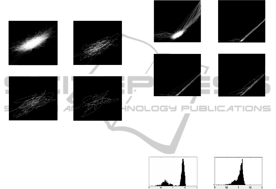
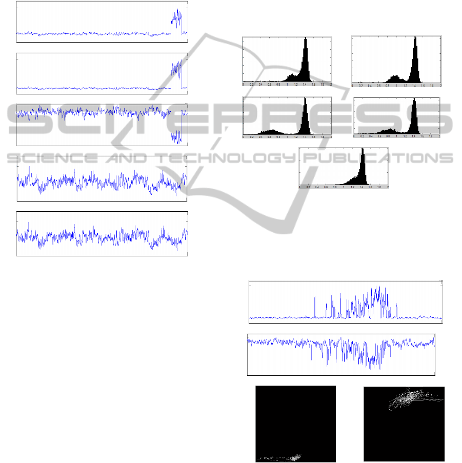
(a) (b)
Figure 12: Histograms of the fractal dimensions calculated
with filter window length on phase plot of number of
source ports for 7000 aggregated samples with a time lag
of 5000 for network traffic containing both normal and
attack traffic: (a) with 10 point low pass filter and (b) with
50 point low pass filter.
For the attack signals the phase plots in Figure 14
show moderate fractal dimensions for the middle
ranges of time lags (100 to 1000) samples, and then
a dramatic reduction at time lags of 5000. Figure 15
shows the histograms of the fractal dimension
calculations for a time series with known attack
signals embedded, and note the general separation of
a lower fractal dimension hump between 0.5 and 1.0,
which contains the attack signals, and then the
higher amplitude, and higher fractal dimension
hump in the histogram for the background data. As
can be expected from Figure 14, there are significant
sections of these time series where for the lower
time lags there would be overlaps in the fractal
SECRYPT 2011 - International Conference on Security and Cryptography
84
dimensions of the attack signals with the normal
background signals as shown in Figure 16. The 5000
sample lag time sequences had no high amplitude
fractal dimensions during any of the attack periods
which results in a more distinct lower fractal
dimension peak in the histogram in Figure 15 (f)
Amplitude
Amplitude
Delta Amplitude Delta Amplitude
(a) (b)
Amplitude
Amplitude
Delta Amplitude Delta Amplitude
(c) (d)
Amplitude
Amplitude
Delta Amplitude Delta Amplitude
(e) (f)
Figure 13: Exploring effects of time lag in phase plot for
number of source ports during normal traffic: (a) time lag
of 1 sample (f
info
=0.68), (b) time lag of 10 samples (f
info
=1.40), (c) time lag of 100 samples (f
info
=1.43), (d) time
lag of 500 samples (f
info
=1.46), (e) time lag of 1000
samples (f
info
=1.34), and (f) time lag of 5000 samples (f
info
=1.30).
The effects of shorter time lags can possibly be
mitigated if the system were designed to detect the
immediate onset of the attack since the transitions
from normal traffic to attacks result in an immediate
and dramatic change in fractal dimension; however,
there is also the chance of higher false alarm rates
from single amplitude spikes. Using a longer time
lag can allow the system to track the existence of the
attack signal for a longer period of time before
declaring an attack detection, which would
dramatically reduce the system false alarm rate.
Likewise the shorter time lags will reduce the ability
to continue to detect the presence of a longer
duration attack since the phase plot will begin to
exhibit multi-fractal behavior as shown in the phase
plots in Figure 16 which may fool a system into
thinking the attack is over.
Amplitude
Amplitude
Delta Amplitude Delta Amplitude
(a) (b)
Amplitude
Amplitude
Delta Amplitude Delta Amplitude
(c) (d)
Amplitude
Amplitude
Delta Amplitude Delta Amplitude
(e) (f)
Figure 14: Exploring effects of time lag in phase plot for
number of source ports during an attack: (a) time lag of 1
sample (f
info
=0.79), (b) time lag of 10 samples (f
info
=1.29), (c) time lag of 100 samples (f
info
=1.05), (d) time
lag of 500 samples (f
info
=1.23), (e) time lag of 1000
samples (f
info
=1.18), and (f) time lag of 5000 samples (f
info
=0.81).
(a) (b)
(c) (d)
(e) (f)
Figure 15: Histograms of the fractal dimensions of phase
plots calculated with varying time lags for attack traffic:
(a) time lag of 1 sample, (b) time lag of 10 samples, (b)
time lag of 100 samples, (c) time lag of 500 samples, (e)
time lag of 1000 samples), and (f) time lag of 5000
samples.
STUDY OF THE PHENOMENOLOGY OF DDOS NETWORK ATTACKS IN PHASE SPACE
85
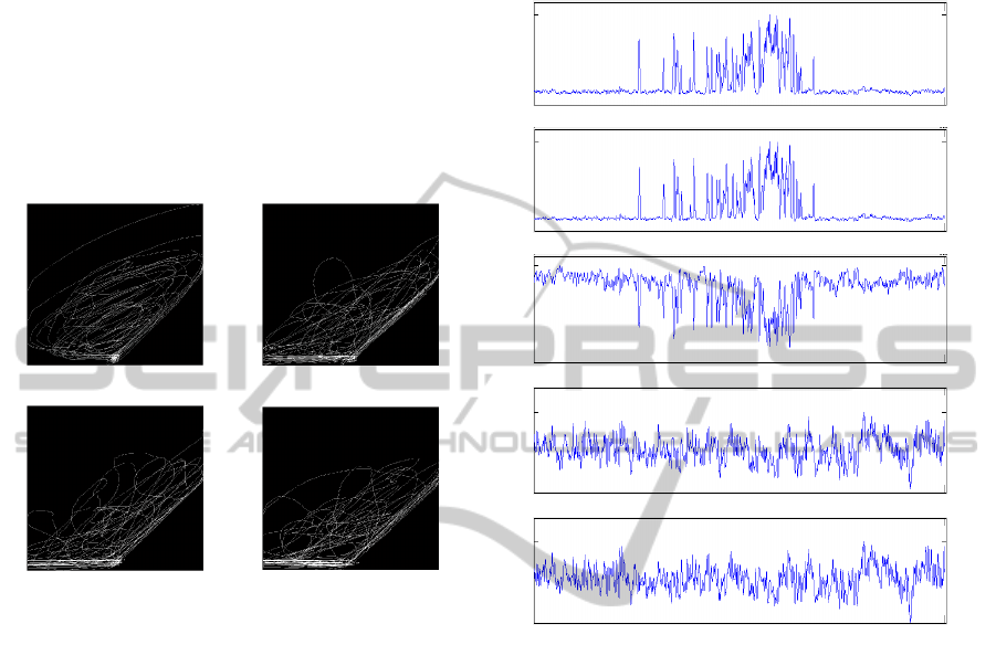
Figure 18 provides the details of the address-
based attacks. Notice again the direct correlation
between the number of source and destination
addresses attempted within the aggregation window
as can be seen in Figure 18 (a) and (b). Notice the
direct correlation of the drop in bytes within the
packets aggregated as is shown in Figure 18 (c).
Also note that during address-based attacks the
number of ports (both source and destination)
identified in the aggregated packet traffic resembles
normal network traffic as can be seen in Figure 18
(d) and (e).
Amplitude
Amplitude
Delta Amplitude Delta Amplitude
(a) (b)
Amplitude
Amplitude
Delta Amplitude Delta Amplitude
(c) (d)
Figure 16: Phase plots for potential detection errors in
attack signal traffic due to varying lag times: (a) 10
sample lag (f
info
=1.49), (b) 100 sample lag (f
info
=1.45),
(c) 500 sample lag (f
info
=1.45), and (d) 1000 sample lag
(f
info
=1.42).
6 STRUCTURE OF ATTACK
SCENARIOS
There are a number of ways in which a DDOS attack
can be orchestrated. The first type, which has been
used for the examples throughout the paper are the
port attacks where the attacker is using large
numbers of source ports and attempting to connect
to a correspondingly large number of destination
ports. The characteristics of the number of ports
during the attack seen can be seen in Figure 17 (a)
and (b). Notice the direct correlation of the number
of source ports and destination ports time series.
Another interesting feature is the corresponding drop
in the number of bytes within the traffic that is
similarly correlated with the number of
source/destination ports as can be seen from Figure
17 (c). Notice also that during port attacks the
number of addresses (both source and destination)
identified in the network traffic resembles normal
network traffic as can be seen in Figure 17 (d) and
(e).
(a)
(b)
(c)
(d)
(e)
Figure 17: Time series for port attacks: (a) time series of
number of source ports, (b) resultant time series of number
of destination ports, (c) resultant time series of number of
bytes, (d) resultant time series of number of source
addresses, and (e) resultant time series of number of
destination addresses.
For developing an attack detection strategy, there
will be a need then to monitor both the aggregated
number of addresses and the aggregated number of
ports in the network traffic. The source and
destination values do not both appear to be required
since they are well correlated. One interesting
observation is that the numbers of bytes in the
aggregated traffic are directly correlated with either
attack, which has been exploited by a number of
researchers who used number of bytes per
aggregation window for their detection scheme.
Consequently, we may also be able to only exploit
the aggregated number of bytes in the network
traffic for attack detection, where any sudden
changes in the fractal value of the number of bytes
then corresponds to a probable attack scenario.
Unfortunately, only monitoring the number of
SECRYPT 2011 - International Conference on Security and Cryptography
86
aggregated bytes does not appear to be an optimal
solution as can be seen in the structure of the
histograms of the fractal dimensions shown in
Figure 19. In these histograms, we have integrated
the values of the fractal dimensions of phase plots of
incoming network traffic collected over an entire
afternoon of the University of Michigan- Flint when
there were known external attacks.
(a)
(b)
(c)
(d)
(e)
Figure 18: Time series for address attacks: (a) time series
of number of source addresses, (b) resultant time series of
number of destination addresses, (c) resultant time series
of number of bytes, (d) resultant time series of number of
source ports, and (e) resultant time series of number of
destination ports.
The separability of the number of aggregated
ports from normal to attack traffic shown in Figure
19 (c) and (d) is significantly better than the
separability of the number of aggregated bytes
shown in Figure 19 (e). Likewise, the number of
aggregated source and destination addresses shown
in Figure 19 (a) and (b) appears slightly better than
that for the byte traffic.
The underlying cause of the number of bytes
being inferior data to analyze when compared to the
number of ports or addresses can be seen in
Figure 20
where we provide a snapshot of an attack traffic
segment showing the aggregated number of source
ports,
Figure 20 (a), and the aggregated number of
bytes traffic time series,
Figure 20 (b). The
corresponding phase plots for these time series are
provided in
Figure 20 (c) and (d), with the
corresponding fractal dimensions provided, and
where the increased fractal nature of the byte traffic
during the attack is clearly visible. This relatively
greater fractal value of the byte information
translates into the peak corresponding to attack
traffic in Figure 19 (e) being shifted significantly to
the right (into the normal traffic peak and above the
fractal value of 1.0). This thereby reduces the quality
of the number of bytes as a measure for detecting the
transition from non-chaotic to chaotic signals.
(a) (b)
(c) (d)
(e)
Figure 19: Histograms of the fractal dimensions of phase
plots for an afternoon of network traffic during period of
known attacks: (a) number of source addresses, (b)
number of destination addresses, (c) number of source
ports, and (d) number of destination ports, and (e) number
of bytes.
(a)
(b)
Amplitude
Amplitude
Delta Amplitude Delta Amplitude
(c) (d)
Figure 20: Comparison of detectability of port information
versus byte information: (a) time series of number of
source ports, (b) time series of number of bytes, (c) phase
space for port information (f
info
= 0.61), and (d) phase
space for byte information (f
info
= 1.15).
STUDY OF THE PHENOMENOLOGY OF DDOS NETWORK ATTACKS IN PHASE SPACE
87

In summary, based on the fractal dimension
histograms in Figure 19 the best separability can be
provided if the aggregated number of destination
addresses (shown in Figure 19 (b)) and the
aggregated number of source ports (shown in Figure
19 (c)) are both monitored. The other signal
parameters provide no additional information and
have generally lower separability of normal network
traffic from attack traffic.
7 CONCLUSIONS
This paper presented an approach to detecting
Distributed Denial of Service attacks using fractal
analysis of the phase space trajectories of the
incoming network traffic. The paper demonstrated
the key differences in behavior of attack traffic and
normal network traffic when analyzed in phase
space. The paper demonstrated the differences in the
characteristics of port and addresses flooding
attacks, and also demonstrated a negative correlation
of the aggregated number of bytes relative to the
aggregated number of ports or addresses referenced.
The paper demonstrates these concepts on actual
network traffic incoming to the University of
Michigan-Flint when it was under a test attack from
the University of Michigan-Ann Arbor.
The results highlighted in the paper demonstrate
there is significant separability between normal
traffic and network traffic when analyzing the
aggregated number of source ports and the
aggregated number of destination addresses. The
paper defined an optimal set of values for the key
parameters related to analyzing these signals in
phase space, namely: (i) the length of the
aggregation window, (ii) the length of the data
analysis window, (iii) the length of low-pass filter,
and (iv) the time lag between samples used to build
the phase space trajectories. These values can be
used to develop an embedded DDOS detection
algorithm in network routers. The paper
demonstrated the efficacy of using the Information
Dimension measure for detecting the changes in the
fractal nature of the phase space trajectories of the
normal and attack traffic. Future work will be
directed at implementing a detection and attack
packet removal algorithm based on the fractal
dimension of the incoming signals and developing
complete Receiver Operating Characteristics (ROC)
curves.
ACKNOWLEDGEMENTS
The authors would like to thank Dr. Stephen Turner,
Anthony Wingett from the Computer Science,
Engineering, and Physics department, and Josh
Weber and the entire University of Michigan-Flint
Information Technology Services organization for
assisting in the data collection process.
REFERENCES
Hu, J. Gao, and N. S. Rao, 2007. Defending against
internet worms using a phase space method from
chaos theory. In SPIE Proceedings # 6570, Data
Mining, Intrusion Detection, Information Assurance,
and Data Networks Security, SPIE.
M. Li, Y-Y Zhang, and W. Zhao, 2008. A practical
method for weak stationarity test of network traffic
with long-range dependence. In Proceedings of the 8th
WSEAS International Conference on Multimedia
Systems and Signal Processing, IEEE.
H. Liangxiu, C. Zhiwei, C. Chunbo, and G. Chuanshan,
2002. A new multifractal network traffic model. In
Chaos, Solitons and Fractals, Elsevier.
M. Masugo, 2002. Multi-fractal analysis of IP-network
traffic based on a hierarchical clustering approach. In
Communications in Nonlinear Science and Numerical
Simulation, Elsevier.
M. Li and W. Zhao, 2008. Detection of variations of local
irregularity of traffic under DDOS flood attack. In
Mathematical Problems in Engineering, Hindawi.
D. Gregg, W. Blackert, D. Heinbuch, and D. Furnanage,
2001. Assessing and quantifying denial of service
attacks. In Proceedings IEEE Military
Communications Conference, IEEE.
M. Li, 2006. Change trend of averaged Hurst parameter of
traffic under DDOS flood attacks. In Computers &
Society.
A. Piskozub, 2002. Denial of service and distributed
denial of service attacks, In Proceedings of
International Conference on Modern Problems of
Radio Engineering, Telecommunications and
Computer Science, IEEE.
Y. Xiang, Y. Lin, W. L. Lei, and S. J. Huang, 2004.
Detecting DDOS attack based on network self-
similarity. In IEE Proc. Communications, IEE.
L. Limwiwatkul and A. Rungsawang, 2004. Distributed
denial of service detection using TCP/IP header and
traffic measurement analysis. In Proc. International
Symposium on Communications and Information
Technologies, IEEE.
A. Mitrokotsa and C. Douligeris, 2005. Detecting denial of
service attacks using emergent self-organizing maps.
In Proc. IEEE International Symposium on Signal
Processing and Information Technology, IEEE.
G. Oke, G. Loukas, and E. Gelenbe, 2007. Detecting
denial of service attacks Bayesian classifiers and
SECRYPT 2011 - International Conference on Security and Cryptography
88

random neural networks, In Proc. IEEE International
Fuzzy Systems Conference, IEEE.
G. Loukas and G. Oke, 2007. A biologically inspired
denial of service detector using the random neural
network, In Proc. IEEE International Conference on
Mobile Adhoc and Sensor Systems, IEEE.
M. F. Rohani, M. A. Maarof, A. Selamat, and H. Kettani,
2007. Uncovering anomaly traffic based on loss of
self-similarity behavior using second order statistical l
model, In International Journal of Computer Science
and Network Security.
L. Feinstein, D. Schnackenberg, R. Balupari, and D.
Kindred, 2003. Statistical approaches to DDOS attack
detection and response, In Proceedings of the DARPA
Information Survivability Conference and Exposition,
IEEE.
H. O. Peitgen, H. Jurgens, and D. Saupe, 1992. Chaos and
Fractals, Springer.
J. L. P. Velaquez, 2005. Brain, behaviour, and
mathematics: are we using the right approaches? In
Physica D, Elsevier.
T. Tel and M. Gruiz, 2006. Chaotic Dynamics,
Cambridge.
J. Theiler, 1990. Estimating Fractal Dimension, In Journal
Optical Society of America, OSA.
J. P. Eckmann and D. Ruelle, 1985. Ergodic theory of
chaos and strange attractors, In Reviews of Modern
Physics, APS.
W. Kinsner, 2005. A unified approach to fractal
dimensions, In Proc. IEEE Conf. on Cognitive
Informatics, IEEE.
A. J. Roberts, 2005. Use the information dimension, not
the Hausdorff, In Journal of Nonlinear Sciences,
Springer.
M. T. Rosenstein and J. J. Collins, 1994. Visualizing the
effects of filtering chaotic signals, In Computers &
Graphics, Elsevier.
H. Korn and P. Faure, 2003. Is there chaos in the brain? II.
Experimental evidence and related models, In C.R.
Biologies, Elsevier.
STUDY OF THE PHENOMENOLOGY OF DDOS NETWORK ATTACKS IN PHASE SPACE
89
