COMPARATIVE ANALYSIS OF THREE TECHNIQUES
FOR PREDICTIONS IN TIME SERIES HAVING
REPETITIVE PATTERNS
Arash Niknafs
1
, Bo Sun
1
, Michael M. Richter
1
and Günther Ruhe
1, 2
1
Department of Computer Science, University of Calgary, Calgary, Alberta, Canada
2
Department of Electrical and Computer Engineering, University of Calgary, Calgary, Alberta, Canada
Keywords: Data mining, Piecewise linear regression, Split points, Prediction.
Abstract: Modelling nonlinear patterns is possible through using regression (curve fitting) methods. However, they
can be modelled by linear regression (LR) methods, too. This kind of modelling is usually used to depict
and study trends and it is not used for prediction purposes. Our goal is to study the applicability and
accuracy of piecewise linear regression in predicting a target variable in different time spans (where a
pattern is being repeated).
Using moving average, we identified the split points and then tested our approach on a real world case
study. The dataset of the amount of recycling material in Blue Carts in Calgary (including more than 31,000
records) was taken as a case study for evaluating the performance of the proposed approach. Root mean
square error (RMSE) and Spearman rho were used to evaluate and prove the applicability of this prediction
approach and evaluate its performance. A comparison between the performances of Support Vector
Machine (SVM), Neural Networks (NN), and the proposed LR-based prediction approach is also presented.
The results show that the proposed approach works very well for such prediction purposes. It outperforms
SVM and is a powerful competitor for NN.
1 INTRODUCTION
In many regression problems, we cannot fit one
uniform regression function to thedata because the
functional relationship between input and target
variables changes at certain points of the domain
(Kuchenhof, 1996); these points are usually referred
to as split points.
Linear regression (LR) is one of the regression
models but a single LR model is not appropriate for
long-term forecast of highly varying and deviant
time series. This is why the family of LR models are
usually used for data interpolation and data
reduction. For example piecewise linear regression
(PLR) has been used in many works for modeling,
observation and then description of medical facts
(Loesch et al., 2006).
PLR is generally used in applications where the
modeling of the target variable by a single line is too
inaccurate and not representative. In this paper we
intend to study the applicability of PLR in prediction
problems where such non-linear patterns are being
repeated periodically over time.
The structure of the rest of the paper is as
follows. In Section 2 we talk about the related work.
Section 3 discusses the background and methods
used. The problem statement and the proposed
solution are illustrated in Section 4 and Section 5,
respectively. Then the solution is evaluated in a case
study in Section 6 –where the experimental results
are also presented. Finally, a few conclusions are
drawn in Section 7.
2 RELATED WORK
Some papers such as (Brown et al., 1975) question
and study the time-constancy of linear regression
models. Kalaba et al. (1989) suggests that the
regression coefficients evolve slowly over time. That
is why it is very common in forecasting time series,
to consider basing the forecasts only on the most
recent version of a time series model rather than on a
model built from the entire series; and that’s because
177
Niknafs A., Sun B., M. Richter M. and Ruhe G..
COMPARATIVE ANALYSIS OF THREE TECHNIQUES FOR PREDICTIONS IN TIME SERIES HAVING REPETITIVE PATTERNS .
DOI: 10.5220/0003463601770182
In Proceedings of the 13th International Conference on Enterprise Information Systems (ICEIS-2011), pages 177-182
ISBN: 978-989-8425-53-9
Copyright
c
 2011 SCITEPRESS (Science and Technology Publications, Lda.)

the recent past contains more information about the
immediate future than the distant past (Guthery,
1974).
There are two concerns regarding PLR that we
are going to address in this paper. First, PLR is
generally used to observe patterns and describe
trends in datasets (e.g. trends in natural phenomena
in medical or biomedical fields of research) and not
used for predictions. Second, in common piecewise
regression approaches, it is only the information
about the input space that is used for partitioning the
data (identifying the split points) (Nusser et al.,
2008). Nusser et al. (2008) for the first time, did the
partitioning using the target variable. The authors in
that paper suggest that ignoring the target variable
and clustering the input data for partitioning the
space is an insufficient strategy in two cases: (a)
“where the data points cannot be distinguished
within the input space”; (b) in regions of high data
density in real-world application problems. These
regions usually correspond to operating points of the
system which are not necessarily appropriate for
partitioning the input space.
Some researches addressed the partitioning of
the data space by considering the values of the target
variable. For example Hathaway and Bezdek,
(1993), Ferrari-Trecate, (2002), Höppner and
Klawonn, (2003) use clustering for this purpose.
From an application point of view, we found out
that there has been a similar work by (Jahandideh et
al 2009) but their PLR model was completely
different from that of ours. In (Jahandideh et al
2009) the goal was devoted to offer a suitable model
to predict the quantity (rate) of medical waste
generation. They used NNs and (Multiple Linear
Regression) MLR models. Their results indicate that
the ANNs model show absolutely lower error
measure compared to the MLR model. Based on
those results, NNs indicated superiority in assessing
the quality in term of accuracy.
In this paper, we incorporate the information
about the target variable into the process of split
(break) point identification in piecewise linear
regression modeling and then use the PLR for long-
term forecasting of time series. An important factor
in many fields of application where transparency and
understandability are highly required in order to
evaluate the proposed solutions by the experts of
that field is the interpretability of the solution
(Nusser et al., 2008). Using moving average, our
proposed solution is very easy to be understood and
interpreted by the experts of other fields where little
mathematical knowledge is required. The need for
this kind of prediction and modeling has been
always there in the City of Calgary but has been
mainly addressed intuitively.
3 BACKGROUND
We used two of the commonly used methods -the
performance of which have been usually compared
to each other in the literature (Fischer, 2008, Sikka
et al., 2010)- to model and forecast time series.
These methods are PLR and SVM. In this paper, we
propose an approach to time series predictions using
PLR and then compare its performance with SVM.
The results are also compared to the results of a
Perceptron NN predictions (NN is popular in
forecasting time series).
We chose SVM because it is well known that
SVM approach works well for pattern recognition
problems and for estimating real-valued function
(regression problems) from noisy sparse training
data (Cherkassky and Ma, 2005). Therefore it is a
good competitor for PLR. This means that it allows
for a good evaluation of the proposed PLR
prediction method through comparing its
performance with that of SVM.
Definition (PLR, Ferrari-Trecate, 2002):
Suppose X is the whole input space in the n-
dimensional space ℝ

. Suppose






are disjoint
regions of X, where 

⋂

= ∅ (, = 1,2,…,)
and ∪




=. The PLR is to determine a
continuous piecewise linear regression function
: → ℝ with a linear behavior in each 

.
The idea of SVM was first developed in (Cortes
and Vapnik, 1995). It is a useful technique for data
analysis and usually used for classification and
regression analysis. SVM maps the original input
 onto a higher dimensional feature space  by a
(potentially non-linear) function 
(
.
)
:→, where
 is a point in the input space .
We use a two layer feed-forward Perceptron
neural network. It has a single output and 6 real-
valued inputs. The idea is to generate the output
using a linear combination of inputs according to the
input weights and then possibly putting the output
through some nonlinear activation function;
mathematically this can be written as (Honkela,
2001):
=(



+)=(


+)


(1)
Where W denotes the vector of weights, X is the
vector of inputs; b is the bias and φ is the activation
function. In the original Perceptron a Heaviside step
function was used. But now the activation function
ICEIS 2011 - 13th International Conference on Enterprise Information Systems
178

is often chosen to be the logistic sigmoid
1/(1 + 

) or the hyperbolic tangent ℎ().
In our case study we set both the learning rate
and the momentum to 0.5. Error epsilon is 1.0E-5
and there are 500 training cycles in which the
learning rate decreases. This is called decay is meant
to avoid over fitting.
4 PROBLEM STATEMENT
Imagine a nonlinear pattern in a time series where
the values of the target variable follow a periodical
pattern. If in each period the pattern can be divided
into smaller time intervals where it can be modeled
by a linear function, then this nonlinear function can
be approximated using a set of linear functions
(Niknafs et al, 2011). An example of such time
series can be seen in Figure 3. Another advantage of
this type of modeling is that it provides easier
interpretability for the experts in different areas. But
our goal is not just modeling the data pattern but
also using PLR to make predictions in both near and
distant future.
LR is usually preferred for data reduction, data
modeling, and data interpolation. Predicting the
closest future points is also another application of
LR. However, we intend to use PLR for both
modeling and predicting the near and distant future
points in a periodical time series -which can be
modeled by LR in smaller time spans in each period.
Beside a solution for applying PLR in this type
of prediction, one has to think of a way of finding
the split points in each of the periods, too.
In other words, we are looking for the set of
disjoining points or split points like 

∈ ℝ,(=
1,2,…, − 1) among the values of the target
variable. Between every two consecutive split
points, the representing points in the input space can
be classified into one class like 

. Therefore we will
have S classes (






) in the input space, where
holds 

⋂

=∅ and ∪




= (Niknafs et al,
2011)
At each of the classes in X, a line can represent
the behavior of the target variable: 

:

→ℝ. We
are studying the special case where one or more of
these lines are being repeated in the time series with
a time period of ,( ∈ ℕ   <
S/2) with slight
differences in the slope. Knowing the  we will be
able to predict a point in future located in , by
using the most recent corresponding line in
(
−
1
)
 where ∈ℕ. The following section (Section 5)
describes our solution approach.
5 SOLUTION APPROACH
5.1 Dataset
We received and processed the daily transaction
records (since April, 2009) of recyclables collected
from Blue Carts -carts in residential places where
residents put the recyclable wastes- from the WRS at
the City of Calgary. This dataset contains the details
about the amount of different recyclables delivered
at the landfills by each truck in each day.
The amount of recyclables is greatly influenced
by the changes in the seasons as well as changes in
weekdays. Thus, in the dataset we split the Date
attributes into three attributes: month, week number
and weekday. Finally, the dataset was structred as
shown in Figure 1. The attributes are Month,
Weeknum, Weekday, Date and different Weights,
where B1 to B3 refer to the weights of Blue Cart
recyclables. The numbers 1, 2, and 3, following the
alphabet B correspond to the weight of the full truck
as it enters the landfill, the load weight and the truck
weight, respectively (Niknafs et al, 2011).
Figure 1: Sample data after data pre-processing.
5.2 Data Pre-processing
The raw data contained lots of noises, empty records
and unrelated columns. First, data cleaning was
performed to remove noises and empty records.
Then a review of the attributes was done to delete
those obviously unrelated attributes, e.g. Truck No.
(plate) and specific transaction hours -because the
minimum prediction granularity is for each day.
The next stage was data aggregation. It was
performed to merge multiple records in one day into
one record containing the total amount of material in
that day. Finally, we aggregated the original 31,898
hourly records into 700+ daily records by summing
up different records in one day. Most of our work
was done with RapidMiner (Rapid-I, 2011), which
covers most of the machine learning techniques.
5.3 Split Points Detection
By visualizing the Blue Cart data, after pre-
processing phase, lots of outliers could be easily
observed at the bottom of the plot as shown in
Figure 2. Further investigation indicated that those
outliers mostly occurr during weekends (Saturdays,
Month Weeknum Weekday Date B1 B2 B3
4 17 3 ######### 647.41 500.60 146.81
4 17 4 ######### 813.86 653.40 160.46
4 17 5 ######### 967.28 729.00 238.28
COMPARATIVE ANALYSIS OF THREE TECHNIQUES FOR PREDICTIONS IN TIME SERIES HAVING
REPETITIVE PATTERNS
179

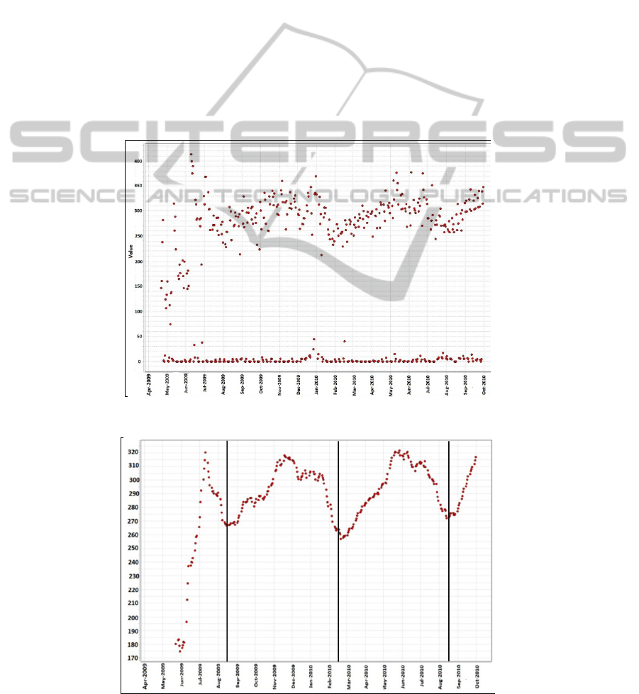
Sunday) and Mondays, and that is because of certain
operational regulations at the City of Calgary. Most
of these data had values equal or very close to zero,
so we eliminated those days from our dataset.
Using a time window of 20 days, the moving
average of the target variable values is calculated. A
curve will be fitted on the data points resulted from
the moving average and then the slope of the curve
is calculated. Using the slope, the extreme points of
the curve are identified. These extreme points are the
split points (

) in this periodical time series, if they
are repeated periodically. The points between these
extreme points in the original dataset are modeled by
linear regression. For predicting the value of the
target variable in a point in future, all we need is to
identify in which corresponding time slot of the
most recent period this point is located. Then we can
choose the line that models that time slot in the time
series history data and use it to predict.
As depicted in Figure 3, there is an instant
increase in the amount of recyclables in Blue Carts
(from late May until early days of July). This is
because the Blue Cart was introduced to different
parts of the city, step by step and in different time
slots. In our approach, we do not take into account
this portion of time because it happens just once for
all and it is not representing the natural behavior of
the target variable.
As depicted in Figure 3, there is a pattern in Blue
Carts data. This pattern repeats every six months.
Those six months can be divided into two
consecutive three months periods. In each of those
three months periods the data points are almost
moving along a single line which is why we used
linear regression to model each of them separately.
Figure 2: Visualization of Blue Cart raw data.
Figure 3: The pattern in the Blue Cart data (moving average) in 2009 and 2010.
ICEIS 2011 - 13th International Conference on Enterprise Information Systems
180

6 EVALUATION (CASE STUDY)
Using two popular measures (RMSE and Spearman
rho) we were able to evaluate the performance of the
proposed approach and also compare it with the
performance of SVM and NN.
6.1 Applying PLR
First we divided our example set into ten parts for a
10-folds cross-validation. Each linear regression
model calculated by RapidMiner is based on the
Akaike criterion for model selection. RapidMiner
provides two types of feature selection methods for a
linear regression model, M5 and Greedy. In this case
study, both of them yielded into almost the same
prediction results (their relative error differed by
0.12%). In general, the Greedy approach that we
used for all experiments performed slightly better
than M5 method.
6.2 Experimental Results
We applied the proposed PLR, as well as SVM and
NN, to predict the daily amount of recyclables for
two different months (July, 2010 and September,
2010). We chose these two months because they are
in two different parts of the repeated pattern, where
the pattern can be modeled by two different lines
(Figure 3). For each of the above mentioned cases,
the history data prior to the target month was used to
train the model.
Using the performance evaluation metrics that
we discussed in Section 5, a comparison between the
performance of SVM, NN, and the proposed PLR
approach is made and presented in Table 1 and
Table 2.
Figure 4 and Figure 5 show the prediction results
for the two months. For both figures, the solid line
depicts the predicted amount of wastes in Blue
Carts, using piecewise linear regression; whereas the
dashed line shows the actual amount. Table 3 and
Table 4 also provide some other evaluation measures
for the proposed PLR approach and give a broader
evaluation view for both predictions in the two
months.
Table 1: Evaluation parameters comparing SVM to the
proposed approach on predictions for September 2010.
RMSE Relative error Spearman rho
LR 10.568 2.67% 0.940
SVM 19.730 5.01% 0.886
NN 10.212 2.56% 0.939
Figure 4: Actual (dashed) vs. PLR predicted (solid)
amounts of material in Blue Cart in July 2010.
Figure 5: Actual (dashed) vs. PLR predicted (solid)
amounts of material in Blue Cart in September 2010.
Table 2: Evaluation parameters comparing SVM to the
proposed approach on predictions for July 2010.
RMSE Relative error Spearman rho
LR 7.590 1.95%
≅1.000
SVM 15.575 4.31% 0.905
NN 9.611 2.43% 0.969
Table 3: Evaluation measures of the proposed approach on
predictions for September 2010.
Performance parameters Blue Cart (PLR)
Root mean squared error 10.568 +/- 0.000
Absolute error 0.749 +/- 5.928
Relative error 2.67% +/- 1.73%
Prediction average 318.862 +/- 15.969
Spearman rho 0.940
Table 4: Evaluation measures of the proposed approach on
predictions for July 2010.
Performance parameters Blue Cart (PLR)
Root mean squared error 7.590 +/- 0.000
Absolute error 5.511 +/- 5.219
Relative error 1.95% +/- 1.72%
Prediction average 281.252 +/- 21.923
Spearman rho
≅ 1.000
COMPARATIVE ANALYSIS OF THREE TECHNIQUES FOR PREDICTIONS IN TIME SERIES HAVING
REPETITIVE PATTERNS
181

7 CONCLUSIONS
We incorporated the information about the target
variable into the process of split point identification
in PLR. The proposed approach is an easily
interpretable method which makes it very
convenient for experts of different fields of research
to use PLR, interpret the patterns and make
conclusions from the forecasts.
In this paper, the application of PLR in seasonal
forecasting in time series with nonlinear patterns is
newly introduced. The applicability and accuracy of
the proposed approach are demonstrated in a case
study at the City of Calgary.
The results show that the proposed approach is a
close competitor of the NN. This close performance
could be attributed to the NN’s non-linear nature
which provides the opportunity to relate different
variables to a target variable.
In this paper, we just based the forecasts on the
most recent linear pattern that corresponds to the
prediction point rather than considering the similar
patterns happening earlier than that. And that’s
because, as we mentioned in Section 1, “the recent
past contains more information about the immediate
future than the distant past”. However, this does not
take into account the possible changes on the
patterns (e.g. changes in the width or position of
time slots). In addition to this limitation of this
study, there is a limitation related to our dataset. The
available history data is limited to almost 2 years,
and that is because the residential Blue Cart program
was just launched in April 2009.
In our future work we intend to study the effect
of integrating a competitive learning method -similar
to the one used in learning the synopsis weight in
competitive neural networks- into the proposed
forecasting piecewise linear regression approach in
this paper. In this way, we will be able to take into
account the variation of the coefficients –which we
talked about in Section 1- in different time slots.
ACKNOWLEDGEMENTS
This research is part of the project CRD #386808-09
supported by NSERC Canada and the City of
Calgary (CoC). Special thanks to Scott Banack from
WRS at CoC for providing the data.
REFERENCES
Brown, R. L., Durbin, J. & Evans, J. M. 1975. Techniques
for Testing the Constancy of Regression Relationships
over Time. Journal of the Royal Statistical Society.
Series B (Methodological), 37, 149-192.
Cherkassky V. & Ma Y. 2005. Multiple Model Regression
Estimation, IEEE Transactions on Neural Networks,
16, 785-798.
Cortes, C. and Vapnik, V. 1995. Support-vector networks.
Machine Learning, 20, 273-297.
Ferrari-Trecate, G., Muselli, M. 2002. A new learning
method for piecewise linear regression In:
International Conference on Artificial Neural
Networks, Springer.
Fischer, M. 2008. Modeling and forecasting energy
demand: Principles and difficulties. In: Proceedings
of the NATO Advanced Research Workshop on
Weather/Climate Risk Management for the Energy
Sector, 207-226.
Guthery, S. B. 1974. Partition regression. Journal of the
American Statistical Association, 69, 945-947.
Hathaway, R. J. & Bezdek, J. C. 1993. Switching
regression models and fuzzy clustering. IEEE
Transactions on Fuzzy Systems 1, 195–204.
Honkela, A. 2001. Nonlinear Switching State-Space
Models, Master’s Thesis, Helsinki University of
Technology, Dep. of Engineering Physics and
Mathematics.
Höppner, F. & Klawonn, F. 2003. Improved fuzzy
partitions for fuzzy regression models. International
Journal of Approximate Reasoning 32, 85–102.
Jahandideh, S. et al. 2009. The use of artificial neural
networks and multiple linear regression to predict rate
of medical waste generation. Waste Management, 21,
2874-2879.
Kalaba, R., Rasakhoo, N. & Tesfatsion, L. 1989. A
FORTRAN program for time-varying linear regression
via flexible least squares. Computational Statistics &
Data Analysis, 7, 291-309.
Kuchenhof, H. 1996. An exact algorithm for estimating
breakpoints in segmented generalized linear models.
University of Munich.
Loesch, D. Z., et al. 2006. Transcript levels of the
intermediate size or grey zone fragile X mental
retardation 1 alleles are raised, and correlate with the
number of CGG repeats. Journal of medical genetics,
44.
Nusser, S., Otte, C. & Hauptmann, W. 2008. An EM-
Based Piecewise Linear Regression Algorithm.
Lecture notes in computer science, 466-474.
Niknafs, A., Sun, B., Richter, M. & Ruhe, G. 2011.
Predictions in Time Series with Repeated Patterns,
Using Piecewise Linear Regression, Technical Report
SEDS-TR-094/2011, University of Calgary.
RAPID-I, http://rapid-i.com/content/view/60/200/,
accessed at December 2010.
Sikka, G., Kaur, A. & Uddin, M. 2010. Estimating
Function points: Using Machine Learning and
Regression Models. In: 2nd International Conforence
on Education Technology and Computer, 52-56.
ICEIS 2011 - 13th International Conference on Enterprise Information Systems
182