
BPEL-TIME
WS-BPEL Time Management Extension
Amirreza Tahamtan, Christian Oesterle, A Min Tjoa
Institute of Software Technology & Interactive Systems, Information & Software Engineering Group
Vienna University of Technology, Favoritenstrasse 9-11/188, A-1040 Vienna, Austria
Abdelkader Hameurlain
Institut de Recherche en Informatique de Toulouse, University Paul Sabatier
Route de Narbonne, 31062 Toulouse Cedex, France
Keywords:
WS-BPEL, Extension, Time, Temporal management, Business process, Design, Execution, Monitoring.
Abstract:
Temporal management and assurance of temporal compatibility is an important quality criteria for processes
within and across organizations. Temporal conformance increases QoS and reduces process execution costs.
WS-BPEL as the accpetd industry standard lacks sufficient temporal management capabilities. In this paper
we introduce BPEL-TIME, a WS-BPEL extension for time management purposes. It allows the definition,
execution and monitoring of business processes with time management capabilities. This extension makes
a fixed, variable and probabilistic representation of temporal constraints possible and checks if the model is
temporally compliant. Our approach avoids temporal failures by the prediction of the future temporal behavior
of business processes.
1 INTRODUCTION
Temporal conformance and compliance are important
quality criteria for business processes and interorga-
nizational workflows. Processes may have deadlines.
The assigned deadlines may be part of the service
level agreement between partners or enforced by law
or organizational policies. It must be ensured that the
right information is delivered to the right activity at
the right time and the process executes in a timely
manner in order to be able to hold the deadlines. Tem-
poral conformance on the one hand increases the QoS
and on the other hand reduces the cost of process ex-
ecution as costly exception handling mechanisms can
be avoided. Temporal management can be used for
three different purposes (Tahamtan, 2009):
• Predictive time management: to predict the pos-
sible temporal behavior of the system and pre-
calculate future possible violations of temporal
constraints.
• Pro-active time management: to detect potential
future violations and raise alarm in these cases
such that counter-measure mechanisms can be tri-
ggered early enough.
• Reactive time management: to react and trigger
exception handling mechanisms if a temporal fail-
ure has already occurred.
Web Services and SOA offer several advantages
for implementation of business processes such as
interoperability, loosely coupling and composition.
WS-BPEL has become the accepted standard for de-
scription end execution of business processes based
on Web Services. In the realm of web services we
mainly talk about two concepts: choreographies and
orchestrations or in the WS-BPEL notation, abstract
and executable processes.
A WS-BPEL executable process or orchestration
is controlled and run by one partner. A partner’s inter-
nal logic and business know-how are contained in his
executable process. Other tasks such as data transfor-
mations, data handling, arithmetic operations and the
actual performed work are as well contained in this
process. An executable process is solely visible to its
ownerand other external partners have no viewon and
knowledge about it. An executable process is a pro-
cess viewed only from the perspective of its owner.
34
Tahamtan A., Oesterle C., Min Tjoa A. and Hameurlain A..
BPEL-TIME - WS-BPEL Time Management Extension.
DOI: 10.5220/0003471000340045
In Proceedings of the 13th International Conference on Enterprise Information Systems (ICEIS-2011), pages 34-45
ISBN: 978-989-8425-55-3
Copyright
c
2011 SCITEPRESS (Science and Technology Publications, Lda.)

On the other hand, a choreography,which is called
abstract process in WS-BPEL, describes business pro-
tocols. An Abstract Process may be used to describe
observable message exchange behavior of each of the
parties involved, without revealing their internal im-
plementation (Alves et al., 2007). An abstract pro-
cess can use all the construct of an executable process
and have the same expressive power but it is not in-
tended to be executed. It has merely a descriptiverole.
An abstract process defines a collaboration among in-
volved partners to reach an overall business goal. It
contains only visible exchanged messages between
partners in course of a business process. An abstract
process has no owner or a super user in charge of con-
trol and all involved partners are treated equally. It is
a process definition from a global perspective shared
among all involved partners (Peltz, 2003).
In order to ensure that cooperating business pro-
cesses are temporally compliant, it must be guaran-
teed that both the tasks performed in executable pro-
cesses and the protocols described in abstract pro-
cesses have a compliant temporal behavior. The Con-
tribution of this paper is an extension of WS-BPEL
called BPEL-TIME (WS-BPEL Time Management
Extension) to ensure temporal compatibility of busi-
ness processes. BPEL-TIME consists of two compo-
nents, a design time component and a run time com-
ponent. The design time component allows the def-
inition of temporal constraints. At design time it is
checked if the model is temporally feasible, i.e. if
there is a solution that satisfies all the temporal con-
straints. If the system is temporally not feasible, it
can be detected at design time and necessary mod-
ifications performed. We calculate a valid temporal
window for each activity in this phase. If an activity
executes within its valid temporal window it is guar-
anteed that the whole process terminates successfully.
The run time component monitors the execution of
the process and informs the process manager if any
deviation from valid temporal windows is detected.
Based on the calculations at design time, the run time
component predicts the future temporal behavior of
the flow and informs the process manager about its
status. Our approach is based on prevention of er-
rors rather than repairing them after their occurrence.
By predicting the behavior of a flow appropriate mea-
sures can be triggered in order to guarantee its suc-
cessful execution. BPEL-TIME offers two different
possibilities: an interval-based and a probabilistic ap-
proach The interval-based approach allows the def-
inition of fixed and/or variable temporal constraints
such as deadlines and durations. The probabilistic ap-
proach enables a probabilistic representation of tem-
poral constraints and takes also branching probabili-
ties into account.
2 MODEL DESCRIPTION
For modeling and calculation of temporal plans of
WS-BPEL executable and abstract processes three
types of constraints have to be considered:
• Implicit Constraints are derived implicitly from
the structure of a process, e.g. an activity can start
execution if and only if all of its predecessors have
finished execution. This kind of constraints also
can be referred to as structural constraints.
• Explicit Constraints, e.g. assigned deadlines,
can be set explicitly by the process designer or
enforced by law, regulations or business rules.
• Dependencies with other Processes may impose
a temporal restriction on a process. It is not
enough to perform a temporal analysis in isola-
tion. The dependencies with other abstract and
executable processes must also be taken into ac-
count.
The first two constraints are needed to calcu-
late the temporal plan of one single process. The
third constraint must be considered in order to check
the temporal conformance and calculate the temporal
plans of a set cooperating processes. We model the
first two constraints using two different modeling ap-
proaches: the interval-based and the probabilistic ap-
proach. Both models are described in subsections 2.1
and 2.2 respectively.
2.1 Interval-based Approach
The interval-based approach allows modeling of fixed
and variable durations of activities. The duration
of an activity can take any value within an interval
bounded by minimum and maximum durations, e.g.
a.d = [a.d
min
, a.d
max
], where a.d refers to duration of
an activity a. We use upper-bound and lower-bound
constraints (Eder and Panagos, 2001) to model the in-
terval within which the duration of an activity lies.
Lower-bound Constraint identifies the minimum
temporal distance between two events. Let a
be the source event and b the destination event.
lbc(a, b, δ) denotes that between the event a and
the event b at least δ time points must pass.
Upper-bound Constraint identifies the maximum
temporal distance between two events. Let a
be the source event and b the destination event.
ubc(a, b, δ) denotes that between the event a and
the event b at most δ time points can pass.
BPEL-TIME - WS-BPEL Time Management Extension
35

a.d
min
and a.d
max
can be modeled by defining the
minimum and maximum allowed time points between
start event and end event of an activity respectively.
This scenario as depicted in fig. 1, where a.d = [2, 7],
a
s
and a
e
refer to the start event and end event of the
activity a. Obviously an activity can also be assigned
a fixed value, if a.d
min
= a.d
max
. Note that in the rest
of this paper, for the sake of brevity, we do not illus-
trate lbc and ubc as well as start and end events in
the graphs. lbc and ubc are not only used for mod-
eling d
min
and d
max
of activities. They can also be
used for modeling temporal constraints between dif-
ferent activities. For example ubc and lbc can be used
for modeling requirements such as approval or rejec-
tion of an application may take at most one week after
its receipt and sending a notification to the applicant
takes at least three days.
Figure 1: Modeling d
min
and d
max
by lbc and ubc.
As the basic modeling language, we adapt the
model presented in (Tahamtan, 2009). It is a timed ac-
tivity graph or timed graph (Panagos and Rabinovich,
1997) augmented with start and end events for ac-
tivities. Timed graphs are familiar workflow graphs
where nodes correspond to activities and edges to the
dependencies between activities, enriched with tem-
poral information. Fig. 2 shows an example of the
model. All activities have a unique name and two cor-
responding events (start and end events). The other
notions used in the fig. 2 are described in subsec-
tion 2.1.1. Because BPEL-processes are full-blocked
(WMC, 2002), in this work we restrict the graphs to
full-blocked ones, i.e. each split node has a counter-
part join node and vice versa.
2.1.1 Calculation of Temporal Values
For calculation of temporal values, we extend the al-
gorithms developed in our previous works (Eder and
Tahamtan, 2008; Eder et al., 2008). All activities have
durations. a.d denotes the duration of an activity a.
The duration is an interval bounded by minimum and
maximum durations. At the first use of a model an es-
timation of the activity durations, e.g. expert opin-
ion, may be used. Later, workflow logs can be mined
for actual activity durations. An interval in which an
activity may execute is calculated. This interval is de-
limited by earliest possible start (eps-value) and lat-
est allowed end (lae-value). a.eps denotes the eps-
value of an activity a and is the earliest point in time
in which the activity a can start execution. eps-values
reflect the implicit constraints of a flow. a.lae rep-
resents the latest point in time in which an activity
a can finish execution in order to hold the assigned
deadline. lae-values reflect the explicit constraints of
a flow. Both eps and lae values are calculated for best
case and worst case. Best case and worst case identi-
fies the execution of the shortest and longest path of a
flow respectively. a.bc.eps refers to best case eps and
a.wc.eps refers to worst case eps of an activity a. The
same applies to lae-values. eps-values are calculated
in a forward pass by adding the eps-value of the pre-
decessor to its duration. Minimum duration for best
case and maximum durationfor worst case are consid-
ered. For example b.bc.eps = a.bc.eps+ a.d
min
and
b.wc.eps = a.wc.eps+ a.d
max
if an activity a is a pre-
decessor of an activity b. If an activity a has multiple
predecessors, e.g. if activity a is an immediate suc-
cessor of an AND-join or the target node of an lbc,
the maximum of eps-values of predecessors of a and
the lbc is taken into account. The eps-value of the
first activity or the set of first activities are set to 0.
In contrast to the eps-values, lae-values are calcu-
lated in a backward pass by subtracting the lae-value
of the successor from its duration, e.g. a.bc.lae =
b.bc.lae − b.d
min
and a.wc.lae = b.wc.lae− b.d
max
if
an activity b is a successor of an activity a. If an ac-
tivity a has multiple successors, e.g. if activity a is
source of an lbc, the minimum of lae-values of prede-
cessors of a and the lbc is taken into account.
Temporal values of a simple graph are depicted in
fig. 2. Given known activity durations, in addition we
can calculate earliest possible end (epe-values) and
latest allowed start (las-values) for an activity, us-
ing the following formulas: a.epe = a.eps + a.d and
a.las = a.lae− a.d. We refer to eps-values and epe-
values as e-values and to lae-values and las-values as
l-values. In this approach we handle loops as com-
plex activities. For calculation of the temporal plan
at design time we consider only one iteration. Be-
cause the actual iterations of a loop is not known at
design time, its execution is monitored at run time
and process manager receives notifications about the
temporal status of the process. For a more detailed
discussion on calculation of interval-based values and
their algorithms, refer to (Tahamtan, 2009; Eder and
Tahamtan, 2008).
ICEIS 2011 - 13th International Conference on Enterprise Information Systems
36
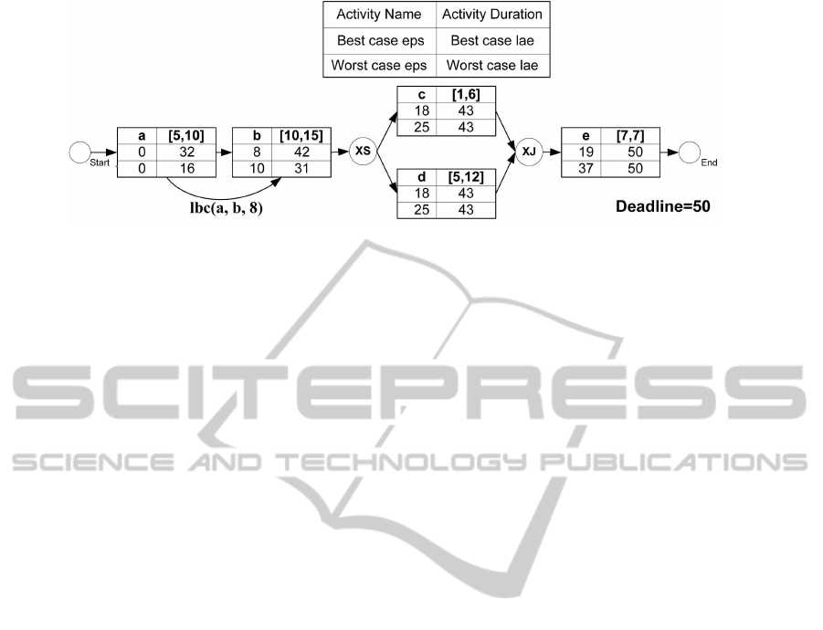
Figure 2: An example of a timed graph with deadline= 50.
2.2 Probabilistic Approach
Fixed or variable duration of activities can be mod-
eled using the interval-based approach. However, in
some use cases one may need to consider branching
probabilities. The probabilistic approach described in
the following subsections caters for probabilistic rep-
resentation of temporal constraints.
2.2.1 Probabilistic Model Description
In order to express variable duration of activities, the
notion of time histograms (Pichler, 2006; Eder and
Pichler, 2002) is used. A duration histogram is a
data structure for representation of the (probabilistic
and variable) duration of basic activities, complex ac-
tivities, subworkflows and workflow itself. A dura-
tion histogram is a tuple (p, d), where p is a prob-
ability and d a duration. For example the proba-
bilistic duration of an activity can be represented as
{(0.1, 10), (0.25, 12), (0.32, 15), (0.33, 20)}. This dura-
tion can be interpreted as follows: the duration of this
activity is with the probability 10%, 10 time points,
with the probability 25%, 12 time points, with the
probability 32%, 15 time points and with the proba-
bility 33%, 20 time points. If a duration histogram
contains any tuples whose time values are the same,
these tuples must be merged by adding the probabil-
ities of tuples with the same duration. A workflow
graph augmented with probabilistic temporal infor-
mation for activities and nodes is referred to as proba-
bilistic timed graph (PTG). Fig. 3 illustrates an exam-
ple of such a probabilistic timed graph. The duration
of activities are given in the table above the graph.
All control nodes have the duration 0. The dead-
line of the workflow is also given in form of a (proba-
bility, duration) tuple. Further, it is assumed that there
is no delay between end of an activity and start of its
successor or the set of its successors. Analogous to
duration histograms (d-histograms), (Pichler, 2006)
defines e-histograms for presentation of e-values and
l-histograms for presentation of l-values. Note that
for probabilistic calculations we do not consider best
and worst case or lbc and ubc.
2.2.2 Histogram Operations
In order to calculate the temporal values, operations
on histograms are necessary. Theses histograms oper-
ations are briefly introduced in this subsection.
The histogram addition generates the carte-
sian product of the tuples of two histograms,
where probabilities are multiplied and time values
are added: {(0.25, 3), (0.75, 5)} + {(0.5, 3), (0.5, 5)} =
{(0.125,6), (0.125, 8), (0.375, 8), (0.375, 10)}. Resulting
tuples with equal time values are aggregated, which
means they are merged by summing up their proba-
bilities: {(0.125, 6), (0.5, 8), (0.375, 10)}.
The histogram subtraction h
1
−h2 is a variation of
the addition, with the only difference that time values
for the resulting tuples are subtracted.
The histogram conjunction also generates
a cartesian product. Again probabilities are
multiplied, but this time the maximum time
value of each tuple-combination determines
the time value of the resulting tuple. There-
fore it is also called the max-conjunction:
{(0.25, 3), (0.75, 5)}
V
max
{(0.5, 3), (0.5, 5)} = {(0.125, 3),
(0.125, 5), (0.375, 5), (0.375, 5)}. Again the final
resulting histogram has to be aggregated, which
results in {(0.125, 3), (0.875, 5)}. A variation of this
operation is the min-conjunction which determines
the time value of the resulting tuple by applying a
minimum-operation.
The weight-operation multiplies all proba-
bilities of a histogram with a given probability:
{(0.25, 3), (0.75, 5)} ∗ 0.25 = {(0.0625, 3), (0.1875, 5)}.
Please note that the weight operation produces an
invalid histogram, as the sum of probabilities is less
than 1.0. Therefore it always appears in combination
with the histogram disjunction, which merges two
weighted histograms:
{(0.0625,3), (0.1875, 5)}
W
{(0.375,3), (0.375, 5)} =
BPEL-TIME - WS-BPEL Time Management Extension
37
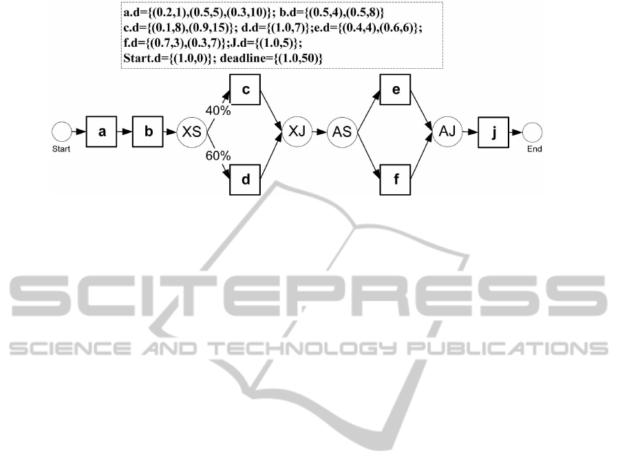
Figure 3: A sample probabilistic timed graph (PTG).
{(0.0.625,3), (0.1875, 5), (0.375, 3), (0.375, 5)}; and the
aggregation which yields to {(0.4375, 3), (0.5625, 5)}.
Both, conjunction and disjunction, are commuta-
tive and associative, therefore they can be extended
to k histograms, e.g.: h = h
1
∨ . . . ∨ h
k
=
W
h
i
, where
1 ≤ i ≤ k.
The histogram comparison is applied for compar-
ing two histograms with each other. Unlike discrete
values, two histograms h
1
and h
2
may partially over-
lap. Thus an expression like h
1
< h
2
can be true and
false at the same time, each at least up to a certain
degree. The comparison of two histograms h
1
and
h
2
with the comparison-operator⊲⊳ ∈ {≤, <, =, >, ≥}
for a given degree 0 ≤ deg ≤ 1 is defined as follows:
h
1
⊲⊳
deg
h
2
=
true : Σp
1
∗ p
2
≥ deg∧ t
1
⊲⊳ t
2
,
∀(p
1
,t
1
) ∈ h
1
, ∀ (p
2
,t
2
) ∈ h
2
false : otherwise
Based on the histograms h
1
and h
2
, depicted in fig. 4,
we can make the following statements: up to a degree
of 0.545, h
1
is greater than h
2
and up to a degree of
0.35, h
1
is equal to h
2
. For instance, the following ex-
pressions are true: h
1
<
0.05
h
2
, h
1
>
0.25
h
2
, h
1
>
0.545
h
2
, and the following are false: h
1
>
0.7
h
2
, h
1
≥
0.9
h
2
.
In order to check the total histogram equality the cer-
tainty degree must be set to 1.0: h
1
=
1.0
h
2
. To ensure
that two histograms have no overlapping regions at
all, they must be compared with the certainty degree
of 1.0: h
1
<
1.0
h
2
or h
1
>
1.0
h
2
.
A relaxed certainty allows for overlapping re-
gions, which might prove useful especially if there
are (extreme) outliers in histograms. For example
imagine that the mean of a histogram h
3
is 5 and it
contains one extreme outlier, the tuple (0.005,1000).
Even with a histograms h
4
that contains much higher
time values, a <-comparison with 100%-certainty al-
ways yields false. Relaxing the certainty-value just by
0.01% will avoid most conformance-conflicts (still,
one day this highly improbable case might occur).
2.2.3 Calculation of Probabilistic Timed Graphs
e-histograms (eps-histograms, epe-histograms) of
nodes of a workflow can be calculated by apply-
ing the forward calculation rules in a topological or-
der. These rules are specified in table 1 according
to the node types. In table 1, node.eps denotes the
eps-histogram of the current node, node.epe its epe-
histogram, node.d the duration histogram of the cur-
rent node, pred.epe identifies the epe-histogram of
the predecessor node, node.Pred the set of predeces-
sor nodes of the current node and p
pred⇒node
identi-
fies the execution probability of the edge connecting
the predecessor node to the current node.
Except for nodes with multiple incoming paths,
i.e. AND-join and XOR-join, the duration-histograms
are summed up to calculate the according e-
histograms. For AND-joins the max-conjunction is
applied because the longest path (or histogram-tuple)
determines the resulting tuple. For XOR-joins, the
histograms of predecessors are weighted with the ac-
cording branching probability and subsequently they
are merged applying the conjunction.
Analogously, for calculation of l-histograms (las-
histograms and lae-histograms) the backward calcu-
lation rules, as specified in table 2, have to be ap-
plied in a backward topological order. In table 2
node.lae refers to the lae-histogram of the current
node, node.las the las-histogram of the current node,
{(1.0, δ)} denotes the assigned deadline, node.d the
duration histogram of the current node, succ.las
identifies the las-histogram of the successor node,
node.Succ the set of successor nodes of the current
node and p
node⇐succ
the execution probability of the
edge connecting the current node with the successor
node.
When reversing the direction of calculation, be-
ginning from the end-node to the start-node, his-
togram subtraction is applied instead of histogram ad-
ICEIS 2011 - 13th International Conference on Enterprise Information Systems
38
0.15
0.50
0.35
10
15
20
0.30
0.70
9
15
0.045 10
15
20
10
15
20
9
9
9
15
15
15
>
>
>
<
=
>
0.350
0.105
0.105
0.150
0.245
t
1
> t
2
: 54.5 %
t
1
t
2
p
1
p
2
p
1
* p
2
t
1
t
2
Histogram h
1
Histogram h
2
t
1
= t
2
: 35.0 %
t
1
< t
2
: 10.5 %
t
1
<= t
2
: 45.5 %
t
1
=> t
2
: 89.5 %
Figure 4: Calculating the values for histogram comparison.
Table 1: Calculation of e-histograms.
type of node node.eps = node.epe =
Start {(1.0, 0)} node.eps+ node.d
End pred.epe node.eps+ node.d
Activity pred.epe node.eps+ node.d
AND-split pred.epe node.eps+ node.d
XOR-split pred.epe node.eps+ node.d
AND-join ∀pred ∈ node.Pred :
V
max
(pred.epe) node.eps+ node.d
XOR-join ∀pred ∈ node.Pred :
W
(pred.epe∗ p
pred⇒node
) node.eps+ node.d
dition. lae-histogram of the end node is initialized
with the assigned deadline. Special rules must be ap-
plied when calculating the l-histograms of the nodes
with multiple outgoing paths: AND-split and XOR-
split. lae-histogram of an AND-split is calculated by a
min-conjunction over its outgoing paths. XOR-splits
are calculated by a weighted disjunction of the outgo-
ing paths. The probabilistic approach provides better
means for handling loops. Again here, loops are han-
dled as complex activities. The number of iterations
can be reflected in durations of the complex activity
with different probabilities. At run time the execu-
tion is monitored. For a more detailed discussion of
the probabilistic approach and some examples, refer
to (Eder et al., 2008).
3 TEMPORAL MANAGEMENT
OF WS-BPEL EXECUTABLE
AND ABSTRACT PROCESSES
The interval-based and the probabilistic approach pre-
sented above can be used to calculate the temporal
plan of one single executable or abstract process in
isolation. However, in order to calculate the tem-
poral plans of a set of cooperating executable and
abstract processes and check their temporal confor-
mance, it is necessary to consider the dependencies
between them. Executable and abstract processes
may be linked in several ways. A typical scenario
(Barros et al., 2005; Decker et al., 2006; Dijkman and
Dumas, 2004) of web service composition assumes
one abstract process shared among several partners
where each partner realizes its parts of the abstract
process in its executable process. The shared abstract
process defines the communication among executable
processes. This scenario is depicted in fig. 5. An exe-
cutable process does not solely contain (a subset of) of
activities of an abstract process rather it may contain
other internal tasks of its owner. (Eder et al., 2007)
provides a technique for checking if the ordering of
the activities in executable and abstract processes is
structurally compliant.
Figure 5: A typical scenario of Web Service composition.
(Eder et al., 2006; Tahamtan and Eder, 2011) in-
troduce other architectures for web service composi-
tion. This architecture is a two layered model where
an abstract or executable process can be an extended
subset of another abstract process. The most im-
BPEL-TIME - WS-BPEL Time Management Extension
39

Table 2: Calculation of l-histograms.
type of node node.lae = node.las =
End {(1.0, δ)} node.lae− node.d
Start succ.las node.lae− node.d
Activity succ.las node.lae− node.d
AND-join succ.las node.lae− node.d
XOR-join succ.las node.lae− node.d
AND-split ∀succ ∈ node.Succ :
V
min
(succ.las) node.lae − node.d
XOR-split ∀succ ∈ node.Succ :
W
(succ.las∗ p
node⇐succ
) node.lae − node.d
portant issue to consider regarding the dependency
between two nodes (abstract and/or executable pro-
cesses) is the greatest common divisor (GCD) of their
activities. GCD identifies the set of common activities
in two nodes. A dependency between two nodes im-
plies that GCD of activities of two nodes is not empty,
i.e. these two nodes have at least one activity in com-
mon. Dependencies between activities are depicted
using links between them as in fig. 5. Fig. 6 depicts
the abstract process C and the executable process O1
in fig. 5. The GCD of two graphs include the activi-
ties Receive request and Reply request. For the sake
of brevity the the executable process O2 is omitted.
If two nodes have no common activities, these two
nodes are temporally independent from each other
and their temporal plans can be calculated in isola-
tion. If GCD of two nodes is not empty these two
nodes affect each other through the common activi-
ties. In this case a cycle of calculation-assignment-
recalculation beginning with the abstract process and
along the all links in the model must be repeated. In
the assignment phase, temporal values of the activi-
ties of GCD are assigned from the source node to the
target node. The assignment is only performed if e-
values of the source node are greater than e-values of
the target node. l-values are assigned if l-values of
the source node are smaller than those of the target
node. In other words an assignment is only allowed
if the current valid execution interval of an activity in
the target node becomes tighter. The concept of as-
signment is depicted in fig. 6. If any temporal value
changes after the assignment, the temporal plan of the
graph must be recalculated as described above. Again
here, current values can be overwritten if newly cal-
culated e-values are greater than current values and
newly calculated l-values are smaller than current l-
values. This cycle is repeated until a stable state is
reached or the conformance condition is violated. A
stable state is reached if no changes is made after as-
signment of values from one node to another. Confor-
mance condition is violated if e-value of an activity
becomes greater than its corresponding l-value. The
top part of the Fig. 6 illustrates the graphs after calcu-
lation of C and O1 and assignment of values from C
to O1. The bottom part of the figure illustrates the val-
ues after recalculation at O1, assignment of the values
from O1 to C. A recalculation at C does not change
the values at C and hence these values are final values.
As you can see the same activities in different graphs
have the same final temporal values. The arrows only
shows the assigned values. For example in the top part
of the figure the e-values of the activity Receive re-
quest in the abstract process C are equal to those in the
executable process O1 and hence not assigned. The
probabilistic approach, as well, uses the same con-
cept for assignment and calculation of temporal plans.
The histogram comparison as described above can be
used for comparing histograms and assignment of val-
ues from one graph to another. The same technique
(calculation-assignment-recalculation) also applies if
there are more than one abstract process present in
the model. In fig. 6 please also note the difference
between deadline and maximum duration (dmax). A
deadline is a point in time whereas maximum dura-
tion is a time period. For example deadline of a pro-
cess may be 15th of July, 12:00 but maximum dura-
tion says that a process can execute for 10 hours after
starting execution.
4 PROTOTYPICAL
IMPLEMENTATION
Our prototype has been implemented based on the
open source softwares Eclipse BPEL designer and
Apache ODE (Orchestration Director Engine). The
prototype consists of two components: A design time
component that allows the definition of cooperat-
ing processes, their dependencies and temporal con-
straints (deadline, activity durations, lower and up-
per bound constraints between activities). The de-
sign time component also checks the temporal sat-
isfiability of the model. It checks if there exists a
solution that satisfies temporal constraints of all pro-
ICEIS 2011 - 13th International Conference on Enterprise Information Systems
40
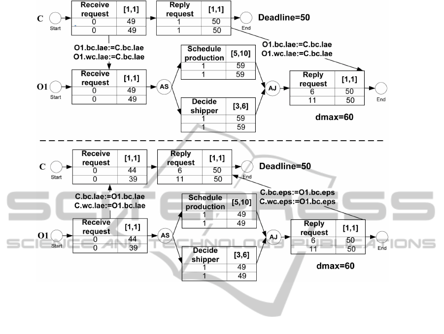
Figure 6: Propagation of values for the same activity in different graphs.
cesses. If such a solution does not exist the user will
be informed which part of the process has temporal
conflicts. In this case process structure or temporal
constraints should be redefined such that the tempo-
ral constraints can be satisfied. Design time compo-
nent calculates a valid temporal window for each ac-
tivity. If activities execute within their valid temporal
window it can be guaranteed that all cooperating pro-
cesses execute and terminate in a temporally compli-
ant way. The run time component monitors the exe-
cution of each activity and checks if it executes within
its valid temporal window. If any deviation is found
the user receives an alarm about the process status.
We use the traffic light model presented in (Eder and
Panagos, 2001). If all activities executes within their
valid temporal window the traffic light is green and
everything is ok. If some activities deviate from their
precalculated valid temporal window but it is still pos-
sible to hold the deadline and satisfy the temporal
constraints (e.g. by executing the shortest path of a
conditional structure) the traffic light turns to yellow.
If some activitiestook longer than expected and in any
case, even in best case scenario, temporal constraints
will be violated, the traffic light turns to red. In this
case the process manager can decide to cancel the
execution prematurely or skip some activities. The
prototype, an installation and troubleshooting guide
and an introduction how to perform basic tasks such
as defining BPEL-process, preparing wsdl-files and
setting up variables can be found on our homepage
(VUT, 2011).
4.1 Design Time Component
The design time component is prototyped under
Eclipse Helios. The required functionalities are im-
plemented under properties as depicted in fig. 7. Af-
ter definition of the structure of the processes, the de-
pendencies between processes can be defined using
the property choreography. A supported process can
be chosen using Select Process. A supported process
identifies processes that have a link to this process,
i.e. their GCD is not empty. This can be an executable
process or another abstract process. The combo box
beneath allows for choosing processes that support
this process. Dependencies can be added or removed.
The result is written in an XML-file called dependen-
cies.xml.
Temporal constraints can be set under Constraints
(see fig. 8). It is possible to set minimum and max-
imum duration of activities and the deadline for the
process. Further it is possible to add and remove op-
BPEL-TIME - WS-BPEL Time Management Extension
41
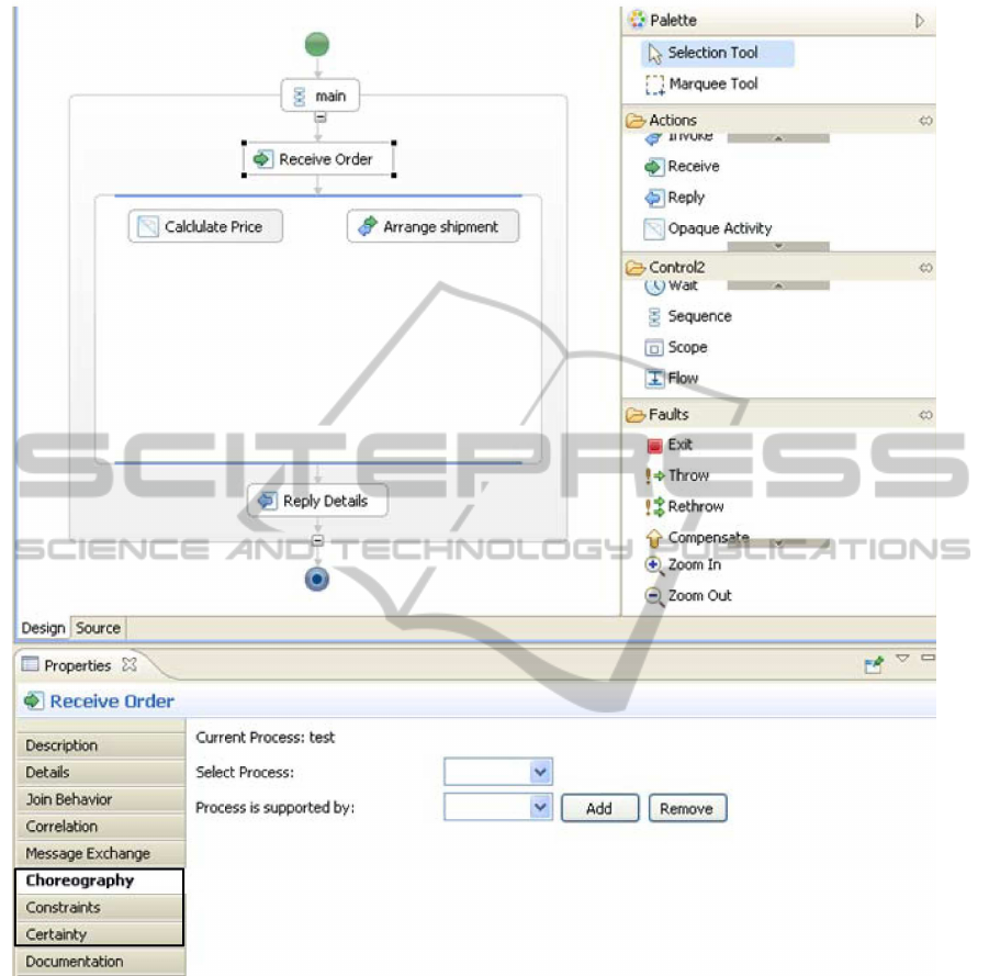
Figure 7: Definition of dependencies between processes.
tional lower and upper bound constraints between ac-
tivities. The right part of the fig. 8 shows the temporal
values of each activity after calculation.
Certainty allows the definition of probabilistic
values: durations of activities and their probabilities
as well as the deadline of the whole process. The
probabilistic temporal values can be calculated by the
Calculate button.
4.2 Run Time Component
The run time component is implemented in Apache
ODE 1.3.4. It monitors the process execution and
checks if activities are executed within their valid
temporal interval. At process instantiation time, an
actual calendar is used in order to transform all time
information which was computed relative to the start
of the flow to absolute time points (Eder et al., 1999).
For every instantiated activity, the calendar e-value is
compared with the start date of the instantiated activ-
ity. In the same way, the mapped calendar l-value is
also compared with the end date of the instantiated
ICEIS 2011 - 13th International Conference on Enterprise Information Systems
42
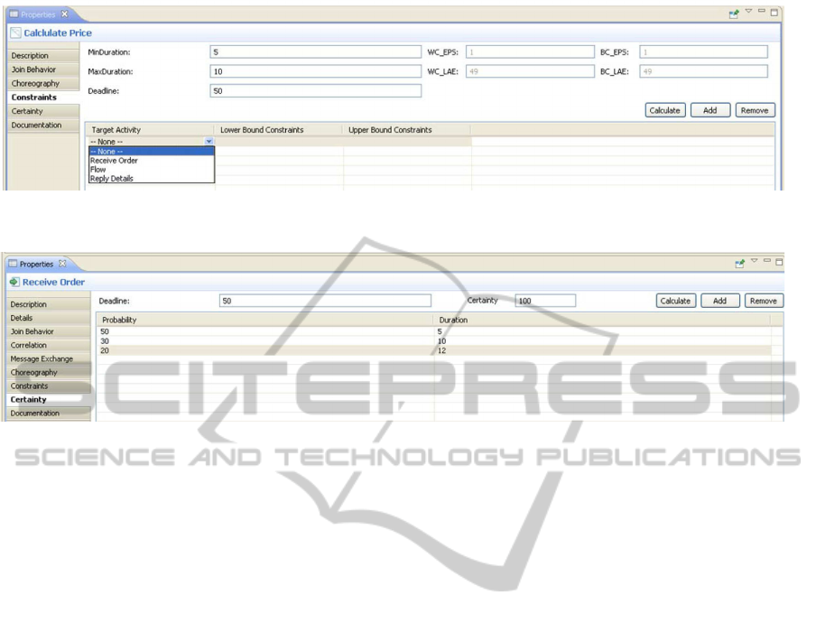
Figure 8: Definition and calculation of interval-based temporal values.
Figure 9: Definition and calculation of probabilistic temporal values.
activity. The traffic light model (Eder and Panagos,
2001) provides an overview for process manager. If
activities execute within their calculated interval at
design time it is guaranteed that all processes remain
temporally compliant. If some activities are delayed
and deviate from their valid temporal window, it is
possible that a deadline be violated. In this case the
traffic light turns to yellow indicating that some ac-
tivities are delayed but it is still possible to finish the
execution in time. The process manager may decide
to force the process to execute the shortest path in or-
der to guarantee the temporal compliance. If activities
are delayed to the extent that future execution in any
case leads to temporal violation, the traffic light turns
to red. In this case, the process manager may want
to cancel execution prematurely in order to reduce the
process execution costs. Fig. 10 shows a screen shot
of the run time component.
5 RELATED WORKS
One of the earliest works on time properties is (Allen,
1983). Allen describes a temporal representation us-
ing the concept of temporal intervals and introduces
a hierarchical representation of relationships between
temporal intervals applying constraints propagation
techniques. This work describes thirteen ways in
which an ordered pair of intervals can be related. Au-
thors in (Eder et al., 1999) present a model for calcu-
lation of temporal plans and propose some algorithms
for calculation and incorporation of time constraints.
(Eder and Panagos, 2001) provides a methodology
for calculating temporal plans of workflows at de-
sign time, instantiation time and run time. It consid-
ers several temporal constraints such as lower-bound,
upper-bound and fixed-date constraints and explains
how these constraints can be incorporated. More-
over, a model for monitoring the satisfaction of tem-
poral constraints at run time is provided. (Eder et al.,
2000) provides a technique for modeling and check-
ing time constraints whilst conditional and parallel
branches are discriminated. In addition, an unfolding-
method for detection of scheduling conflicts is pro-
vided. Marjanovic in (Marjanovic, 2000) represents
the notions of duration space and instantiation space
and describes a technique for verification of temporal
constraints in production workflows. The approach
presented in this paper is complementary to that in-
troduced in (Marjanovic, 2000) in the way that a
temporal plan for execution of all activities is cal-
culated. (Benatallah et al., 2005) uses temporal ab-
stractions of business protocols for their compatibil-
ity and replaceability analysis based on a finite state
machine formalism. Kazhamiakin, Pandya and Pi-
store in (Kazhamiakin et al., 2006b), as well as in
(Kazhamiakin et al., 2006a), exploit an extension of
timed automata formalism called web service time
transition system (WSTTS) for modeling time prop-
erties of web services. The approach presented in
this work can cover cases which can be modeled in
these works and additionally allows the definition of
BPEL-TIME - WS-BPEL Time Management Extension
43

Figure 10: The run time component monitors the execution.
explicit deadlines. This work extends previous works
by addressing the conformance and verification prob-
lem and provides an a priori execution plan at design
time consisting of valid execution intervals for all ac-
tivities of participating abstract and executable pro-
cesses with consideration of the overall structure and
temporal restrictions. The calculated execution plans
can be monitored at run time. (Bettini et al., 2002)
proposes a formalism for representation of quantita-
tive temporal constraints. A consistency service en-
sures the satisfiability of temporal constraints. Au-
thors in (Kallel et al., 2009) propose an approach for
specification and monitoring of relative and absolute
temporal constraints based on XTUS-automata and
Ao4BPEL. In this approach temporal constraints can
be translated into modular aspect code that listens to
activities during the execution of a process. An activ-
ity will be only executed if the temporal constraints
are satisfied. Guermouche et al. in (Guermouche
et al., 2008) study temporal aspects of Web Services.
They differentiate between internal and external tem-
poral constraints. Internal constraints specify a rel-
ative and absolute time period and can be used for
expression of activation and dependency conditions.
External constraints are exposed by the client and the
provider service. They have to be checked before in-
teraction initialization. They infer from internal con-
straints and allow for detection of incompatibilities
of services. Song et al. in (Song et al., 2009) use
petri nets for description and modeling of behavior
and temporal aspects of BPEL processes. The short-
coming of this approach is that only analysis is con-
sidered. Our approach is complementary in the sense
that it allows for analysis and temporal reasoning and
further a BPEL-extension for execution is provided.
6 CONCLUSIONS
Temporal management and consistency are important
quality criteria for business processes. They improve
QoS and reduce costs. WS-BPEL lacks sufficient
time management capabilities. In this work we intro-
duced an extension of WS-BPEL that makes business
processes time aware and overcomes this shortcom-
ing. The user can define different temporal constrain-
ICEIS 2011 - 13th International Conference on Enterprise Information Systems
44

ts, check temporal feasibility and monitor the execu-
tion. The two considered techniques, interval-based
and probabilistic, caters for different needs of the
users in different scenarios.
REFERENCES
Allen, J. (1983). Maintaining knowledge about temporal
intervals. Communications of the ACM, 26(11):832–
843.
Alves, A., Arkin, A., Askary, S., Barreto, C., Bloch, B.,
Curbera, F., Ford, M., Goland, Y., Guzar, A., Kartha,
N., Liu, C., Khalaf, R., Koenig, D., Marin, M., Mehta,
V., Thatte, S., Rijn, D., Yendluri, P., and Yiu., A.
(2007). Web services business process execution lan-
guage version 2.0. Technical report, OASIS.
Barros, A., Dumas, M., and Oaks, P. (2005). A criti-
cal overview of the web services choreography de-
scription language(ws-cdl). Technical report, Busi-
ness Process Trends.
Benatallah, B., Casati, F., Ponge, J., and Toumani, F.
(2005). On temporal abstractions of web service pro-
tocols. In Proc. of CAiSE Forum.
Bettini, C., Wang, X. S., and Jajodia, S. (2002). Tempo-
ral reasoning in workflow systems. Distrib. Parallel
Databases, 11:269–306.
Decker, G., Overdick, H., and Zaha, J. (2006). On the suit-
ability of ws-cdl for choreography modeling. In Proc.
of EMISA’06.
Dijkman, R. and Dumas, M. (2004). Service-oriented de-
sign: A multi-viewpoint approach. Int. J. Cooperative
Inf. Syst., 13(4):337–368.
Eder, J., Gruber, W., and Panagos, E. (2000). Tempo-
ral modeling of workflows with conditional execution
paths. In Proc. of the 11th International Conference
on Database and Expert Systems Applications.
Eder, J., Lehmann, M., and Tahamtan, A. (2006). Chore-
ographies as federations of choreographies and or-
chestrations. In Proc. of CoSS’06.
Eder, J., Lehmann, M., and Tahamtan, A. (2007). Confor-
mance test of federated choreographies. In Proc. of
I-ESA’07.
Eder, J. and Panagos, E. (2001). WfMC WorkFlow Hand-
book 2001, chapter Managing Time in Workflow Sys-
tems. J. Wiley & Sons.
Eder, J., Panagos, E., and Rabinovich, M. (1999). Time con-
straints in workflow systems. In Proc. of the 11th In-
ternational Conference on Advanced Information Sys-
tems Engineering (CAiSE).
Eder, J. and Pichler, H. (2002). Duration histograms for
workflow systems. In Proc. of the IFIP TC8 / WG8.1
Working Conference on Engineering Information Sys-
tems in the Internet Context.
Eder, J., Pichler, H., and Tahamtan, A. (2008). Probabilis-
tic time management of choreographies. In Proc. of
QSWS-08.
Eder, J. and Tahamtan, A. (2008). Temporal conformance
of federated choreographies. In Proc. of DEXA’08.
Guermouche, N., Perrin, O., and Ringeissen, C. (2008).
Timed specification for web services compatibility
analysis. Electron. Notes Theor. Comput. Sci., 3:155–
170.
Kallel, S., Charfi, A., Dinkelaker, T., Mezini, M., and
Jmaiel, M. (2009). Specifying and monitoring tempo-
ral properties in web services compositions. In Proc.
of the Seventh IEEE European Conference on Web
Services.
Kazhamiakin, R., Pandya, P., and Pistore, M. (2006a). Rep-
resentation, verification, and computation of timed
properties in web service compositions. In Proc. of
ICWS 06.
Kazhamiakin, R., Pandya, P., and Pistore, M. (2006b).
Timed modelling and analysis in web service compo-
sitions. In Proc. of ARES06.
Marjanovic, O. (2000). Dynamic verification of temporal
constraints in production workflows. In Proc. of the
Australasian Database Conference.
Panagos, E. and Rabinovich, M. (1997). Predictive work-
flow management. In Proc. of the 3rd Int. Work-
shop on Next Generation Information Technologies
and Systems.
Peltz, C. (2003). Web services orchestration and choreog-
raphy. IEEE Computer, 36(10):4653.
Pichler, H. (2006). Time Management for Workflow
Systems. A probabilistic Approach for Basic and
Advanced Control Flow Structures. PhD thesis,
Alpen-Adria-Universitaet Klagenfurt. Fakultaet fuer
Wirtschaftswissenschaften und Informatik.
Song, W., Ma, X., Ye, C., Dou, W., and Lu, J. (2009). Timed
modeling and verification of bpel processes using time
petri nets. In Proc. of the International Conference on
Quality Software.
Tahamtan, A. (2009). Modeling and Verification of Web
Service Composition Based Interorganizational Work-
flows. PhD thesis, University of Vienna.
Tahamtan, A. and Eder, J. (2011). View driven interorgani-
zational workflows. Int. J. Intelligent Information and
Database Systems, To Appear.
VUT (2011). Vienna university of technology, insti-
tute of software technology and interactive sys-
tems, information & software engineering group.
http://www.ifs.tuwien.ac.at/.
WMC (2002). Workflow process definition interface -
xml process definition language. Technical Report
WFMC-TC-1025, The Workflow Management Coali-
tion.
BPEL-TIME - WS-BPEL Time Management Extension
45
