GROUPING FOR THE CRITERIA BASED DATA BROADCAST
IN WIRELESS MOBILE COMPUTING
John Tsiligaridis
Heritage University, Math and Computer Science, Heritage 3240 Fort Road, Toppenish, WA, 98948, U.S.A.
Keywords: Data broadcast, Scheduling, Mobile computing.
Abstract: Data broadcasting in wireless communication technology can provide mobile financial with location based
services. Data can be reached in any time and place. The server fetches the requests and broadcasts the data
to the air. The broadcast problem including the plan design is considered. A criteria based algorithm can
discover the creation of a full or empty slot Broadcast Plan (BP) with equal spacing of repeated instances of
items. This last property can guarantee the creation of a regular BP (RBP) and enable the servers use a
single or a number of channels so that the users can catch their items avoiding their devices’ waste of
energy. Moreover, the Grouping Dimensioning Algorithm (GDA) based on integrated relations can
guarantee the discrimination of services using a minimum number of channels. The server broadcasting
capability is increased for a single channel operation by the use of the HOL waiting time group (HOL-
WTG) scheduler, providing service priority along with bandwidth adjustment, diminishing the waste of
bandwidth, and minimizing the number of rounds. This proposed work can enrich the server infrastructure
for self-monitoring, self-organizing and channel availability as well. Simulation experiments are provided.
1 INTRODUCTION
The mobile computing is based on the
communication between clients and the large scale
distributed database. An efficient broadcast schedule
program minimizes the client expected delay, which
is the average time spent by a client before receiving
the requested items. The expected delay is increased
by the size of the set of data to be transmitted by the
server. In our approach suitable adjustment of the
server’s bandwidth is made so that the data be
transmitted minimizing the delay (Bertossi et al.,
2004, Kenyon et al. 2000, Bar-Noy et al. 2003). The
memory hierarchy can be constructed so that the
highest levels contain more items broadcasting them
with high frequency while the subsequent levels
contain items that broadcast at lower frequency
(Acharya et al., 1995). Additionally data items are
assigned to different “disks “ (Bdisks) of varying
sizes and speeds and are then broadcasted in the air.
Items stored on faster disks are broadcasted more
often than items on slower disks (Bertossi et al.,
2004), (Acharya et al. 1996). There are many
strategies for the broadcast delivery with two basic
categories (Sumari et al., 2003). In the static
broadcasting the schedule of the program is fixed
(static) even though the contents of a program can
change with time (Bertossi et al., 2004). In the
dynamic broadcasting, both the schedule of
programs and its contents can change and there
exists limited support to handle user’s requests
(Bertossi et al., 2004 ). In (Bowen et al., 1992) data
broadcasting is developed introducing the datacycle.
The server broadcasts more popular items more
frequently to minimize the average access time. In
(Sumari et al., 2003) a new technique for storing
data on disk the “sequence” is developed and
broadcasts them in accordance to their order.
Very long messages delay all the others and the
service rate needs adjustment depending on the size
of the message and the available amount of
bandwidth that the server can provide. To this
direction, the criteria broadcast plan algorithm
(CBPA) is presented which examines the possibility
to get a BP, by discovering the number of times that
an item will be in the cycle, and the construction of
the full BP (CBP). The broadcasted items can be
divided into i sets depending on the items’
popularity. The CBP can be independent of the
number of the serviced sets. We start with the
biggest size set (S
3
, with the least popularity) as the
basis of the button-up planning design and work
203
Tsiligaridis J..
GROUPING FOR THE CRITERIA BASED DATA BROADCAST IN WIRELESS MOBILE COMPUTING.
DOI: 10.5220/0003474402030209
In Proceedings of the 6th International Conference on Software and Database Technologies (ICSOFT-2011), pages 203-209
ISBN: 978-989-8425-76-8
Copyright
c
 2011 SCITEPRESS (Science and Technology Publications, Lda.)

iteratively in order to find the parameters of the
optimal BP. In this work we focused on the
homogenous data (items) and the heterogeneous
having multiple size of the basic packet size (f.i.
512KB). Homogenous data have the same size. The
terms bandwidth and weight are used
interchangeably. The data can be sent by a single
channel or a set of channels.
Finding the number of channels that can send a
group of data providing also the equal spacing of
repeated instances of items could be very interesting
issue. GDA finds directly the minimum number of
channels that make an RBP efficient. The surplus of
the available channels from both grouping
algorithms may be used for another RBP.
The rest of the paper is organized as follows. In
section 2 the Model Description is described. In
section 3 some analytical results with their
conditions are described. In section 4 the CBPA is
developed. In section 5 and 6, the GDA and the
HOL-WTG are developed respectively. Simulation
results are provided in section 7.
2 MODEL DESCRIPTION
2.1 General
Our work is starting from the last level of hierarchy
(the less popular items)we try to find the numbers of
items repetitions according to a set of proposed
algorithms. The condition to have a BP for various
items and numbers of times so that the most popular
items be transmitted within a period is examined.
Our approach can (1) create an innovative
broadcast program design (2) with the RBP it also
provides energy efficient access to items by
minimizing the user average waiting time (AWT).
The time difference between two continual
broadcast slots for the same item is called spacing s
i
of that item i
i
. Equal spacing is when the spacing for
any item of the cycle remains the same. There are
three design strategies: the flat, the skewed, and the
regular (or multi-disk) (Acharya et al., 1995). The
last two are referred as hierarchical design where the
data items are divided into two levels of hierarchy
with the more popular data allocated to the smaller
level. For the flat design a number of data items are
allocated to a channel broadcast regardless of
popularity. In the skewed design more popular data
are broadcasted more frequently (Acharya et al.,
1995). In the regular design there is no variance in
the inter arrival time for each item and we have
equal spacing for all the instances of the items of the
cycle (Acharya et al., 1995). Our goal is to provide a
BP that is regular in order to guarantee the equal
spacing of all the instances of the items of the cycle,
to minimize TT (for all the instances) and make it
more energy efficient. For example, consider that
the spacing for A item is 5, 20 and 50 sec. If the user
starts the listening randomly then he has to wait
probably for various time intervals which cost
battery waste. In the regular plan which provides
equal spacing of 5 sec the random start of listening
until he retrieves the item A can last only 5/2=2.5
sec (on average).
First we develop the criteria based algorithm that
identifies the type and parameters of a BP (CBPA)
that can be produced from a set of users’ items, and
the construction of a full BP (CBP). Secondly, a new
group scheduler based on the HOL waiting time
(HOL-WTG) is introduced in order to guarantee the
queues service priority. The order of service of the
queues is held according to each queue’s HOL item
predefined waiting time.
2.2 The Design of the Relation
The possibility of providing BP (full or not) is
examined iteratively starting from the last level of
hierarchy S
3
. The size of a set stands for S
is
(where
i=1,2,3). It is considered that S
3s
 S
2s
 S
1s
, and
the number of S
3
items will be sent only once while
for the other sets at least twice. We create a set of
relations including their subrelations by considering
items of different size from each set. This is
achieved by finding the integer divisors of S
3s
(k
1
,
k
2
, k
3
,..k
i
…k
n
) and put them at a decreasing order in
an array (ar). Each relation has three subrelations. It
is also assumed that S
2s
, S
3s
are not prime numbers.
For the BP design in case that S
2s
is a prime number,
it is possible to add only one empty slot at the end of
the last major cycle. The next integer number of a
prime is a composite number. This idea helps to
create the BP. The following definitions are
essential:
Definition 1: The size (or horizontal dimension) of a
relation (s_rel) is the number of items that belong to
the relation and it is equal to the sum of the size of
the three subrelations (s_rel=
3
1
_
i
i
s
sub


). The
number (or vertical dimension) of relations (n_rel)
with s_rel define the area of the relations (area_rel).
Example 1: The relation A=(a, b, c, d, f) has the
following three subrelations starting from the end
one; the 3-subrelation (f) with s_sub
3
= 1, the 2-
subrelation (b,c,d) with s_sub
2
= 3, and the 1-
subrelation (a) with s_sub
1
=1. The s_rel=5
ICSOFT 2011 - 6th International Conference on Software and Data Technologies
204

Definition 2: The area of the i-subrelation
(area_i_sub) is defined from its size (s_sub
i
) and
the number of the relations (n_rel) that are selected.
It is given by (s_sub
i
) x (n_rel).
Example 2: From a relation with s_rel=5 and if
n_rel=5 then the area of this relation is 5x 5 .
Hence there are 25 locations that have to be
completed.
Example 3: If two relations are: (1,2,3,5,6,7),
(1,3,4,8,9,10) with s_sub
3
=3, s_sub
2
=2, then : 2-
subrelation
1
=(2,3) and 2-subrelation
2
=(3,4). The last
two subrelations ((2,3),(3,4)) comes from S
2
={2,3,4} having 3 as repeated item.
Definition 3: An BP is full if it provides at least 2
repetitions of items and it does not include empty
slots in the area_rel
Definition 4: The number of items that can be
repeated in a subrelation is called item multiplicity
(it_mu) or number of repetitions (n-rep).
Definition 5: The optimal BP for S
1s
< S
2s
< S
3s
, is
the full BP taken with the maximum effective n_rel (
providing also the maximum items multiplicity for
the subrelations). For optimal BP the most popular
items are transmitted more often. Our full BP is also
optimal BP since the items of S
2
and S
1
are repeated
more than one times.
Definition 6: Integrated relations (or integrated
grouping) are when after the grouping, each group
contains relations with all the data of S
2
and S
1
. This
happens when: ( (2_subrelation) = S
2
)  ( 
(1_subrelation) = S
1
). See example 7 for details.
Definition 7: An FBP is direct when k S
div
and S
2s
|
k (S
2s
<k). It is indirect when k S
div
and k | S
2s
(k>S
2s
)
It is considered that a|b (a divides b) only when b
mod a =0 (f.e. 14 mod 2=0). The relation with the
maximum value of n_rel provides the opportunity
of maximum multiplicity for all the items of S
2
and
S
1
and finally creates the minor cycle of a full BP.
The major cycle is obtained by placing the minor
cycles on line. The S
div
contain all the divisors of
S
3s
. Hence S
dil
={d
1
,d
2
,..,d
n
}.
3 SOME ANALYTICAL RESULTS
FOR BP AND RBP CREATION
A set of Lemmas can discover the possibility of
having a full equal spacing BP. from the sets (S
is
/
i=1,2,3).
Lemma 1: Let us be k any integer divisor of S
3s
. If
k≥S
is
(i=2,3) and S
is
| k then we can take a full direct
BP.
Proof: If k≥ S
is
and S
is
| k => k= S
is
* m (m I )
and any item of S
2s
can be repeated for m times
Hence it_mu
i
= k / S
is
. Since this happens for all the
sets, a full BP can be produced using just the items
of the S
is
.
Example 4: (full BP)Consider the case of: S
1
= {1},
S
2
={2,3}, S
3
= { 4,5,6,7,8,9, 10, 11}. Finding the
integer divisions of S
3s
(=8) which are 4(8/2) and
2(8/4). The n_rel could be 4(8 /2) or 2(8/4). Hence
S
div
= {d1,d2}= {4,2}. If n_rel=4 the format of the
four relations with S
1
could be:
( * * * ..* 4,5), ( * * * ..* 6,7), ( * * * ..* 8,9), ( *
* * ..* 10,11). For n_rel= k =4 then 4>2 and it_mu
i
=2=4/2 it means that there is a full BP for S
2
.
Using again the same for the S
1
we take 4>1 and
it_mu
i
=2=4/1 it means that there is a full BP for
S
1
. One relation of the full, direct could be: (1,2,4,5).
Lemma 2: If k<S
is
(i=2,3) and k | S
is
then we can
take a full indirect BP. In this case the total number
of items (t_n_i
i
) that transferred and the s_sub
i
can
be easily computed.
Proof: If k<S
is
(i=2,3) and k | S
is
then S
is
= k *m (m
I ) and this gives again it_mu
i
=S
is
/k.
Additionally, a predefined it_mu for S
is
can be
defined so that t_n_i
i
= S
is
* it_mu
i
and s_sub =
t_n_i / n_rel.
Example 5: Let’s consider S
1
= 1, S
2
= {2,…,13}, S
3
= {15,…,32} with: S
1s
= 1, S
2s
= 12, S
3s
= 18.
Finding the integer divisors of S
3s
(=18) which are
9(18/2), 6(18/3), 3(18/6). The decreasing order is:
9,6,3. (a) For n_rel=k=9, since 9<12 and 912 only
empty slot BP possibility. (b) Taking the next k
value (k=6), since 6<12 and 6|12 there is a FBP
with it_mu=2, t_n_i=12*2=24, s_sub=t_n_i / k =
24/6=4. Hence the 2- subrelation for the 6 relations
can be: (..,2,3,4,5,..), (..,6,7,8,9..), (..,10,11,12,13,..),
(..,2,3,4,5,..), (..,6,7,8,9,..), (..,10,11,12,13,. ..) having
two repetitions for each item. Hence 1-subrelation =
6, 2-subrelation=4.
Lemma 3: If k<S
is
(i=2,3) and k  S
is
then it is not
possible to take a full BP.
Proof: Because it_mu
i
= k/S
is
 I.
Example 6: Let us consider S
1
= 1, S
2
= {2,3,4}, S
3
=
{5,…,22} with: S
1s
= 1, S
2s
= 3, S
3s
= 18. Finding
the integer divisors of S
3s
(=18) which are 9(18/2),
6(18/3), 3(18/6). Decreasing order 9,6,3. For
n_rel=k=9,since 9>3,(from (1),(2)) with it_mu
3
=3
=9/3 there is a strong 3-subrelation. (1,2,5,6),
(1,3,7,8), (1,4,9,10), (1,2,11,12), (1,3,13,14),
(1,4,15,16), (1,2,17,18), (1,3,19,20), (1,4,21,22). The
BP is an RBP (equal spacing for all the sets), for
GROUPING FOR THE CRITERIA BASED DATA BROADCAST IN WIRELESS MOBILE COMPUTING
205

data of S
2
(period
2
=11) and S
1
(period
1
=3). Using a
single channel for all the data (the relations) you can
take the same average waiting time AWT for the
users interested in data of S
1
and S
2
. For “2” the
AWT
2
=11/2=5.5. Making groups of three relations
and using three channels we get again the same
AWT for the users interested in data of S
1
and S
2
.
On the contrary, for users interested in data of S
3
the
AWT is much longer when a single channel is used
instead of multiple ones.
Taking the next k value (k=6), since 6>3 and
it_mu
2
=2 =6/3 again we get a strong 2-subrelation.
The subrelations are: (1,2,3,5,6,7), (1,3,4,8,9,10),
(1,2,3,11,12,13), (1,3,4,14,15,16), (1,2,3,17,18,19),
(1,3,4,20,21,22). This BP is not equal spacing
because the 2-subrelation
1
=(2,3), and 2-
subrelation
2
=(3,4) have a common item (3).
Obviously for k=3 we take it_mu
1
=1 and it is also a
strong 1-subrelation. The best BP is taken with k=9,
the maximum multiplicity value for S
2
providing
also equal spacing possibility.
4 THE CRITERIA BROADCAST
PLAN ALGORITHM (CBPA)
Our CBPA approach is very different than the
previous ones (Acharya et al.,1995), (Acharya et al.,
1996) and it is based on the creation of the optimum
size of relations of i sets of items, that can cover the
desired number of repetitions (copies) of items. The
broadcasted items can be separated into i sets
depending on their items popularity. The CBPA is
independent of the number of the serviced sets. We
start with the largest size set (S
3s
, with the least
popularity) as the basis of the bottom-up planning
design and we basically find a number of relations
(n_rel) that may provide a full BP. Starting with the
maximum value of n_rel, the CBPA provides plans
of the items distribution from the other two sets
(level by level) for the remainder empty positions of
the relation, in order to complete the kth size
subrelations. The optimum planning is achieved
using a set of two allocation criteria so that to
maximize the number of sending items of the upper
sets (S
2
, S
3
). Additionally the items of the sets are
inserted direct into the queues,without the use of an
intermediate list, and the scheduler start the
servicing. There are three criteria that must be
completed for the selection of the optimum plan:
Criterion 1: It shows the possibility of having a
direct full BP according to Lemma 1. The number of
S
3
data must be allocated into integer number of
relations. The divisors are sorted in decreasing order
(S
div
={d
1
,d
2
,..,d
n
},d
i+1
> d
i
) and for each one, a
number of items n_it (n_it=S
3s
/d
i
) defines the
number of S
3
items in the more right position of the
relation. The rest positions of the relations are
covered with items of S
2
and S
3
using the next
criterion. Details are in examples 5,6.
Criterion 2: It examines the case for indirect full BP
according to Lemma 2. Details are in example 6.
This criterion will be used iteratively in order to find
the numbers of items for each next upper set (level)
in the relations. In case that the size of any set is
less than the n_rel (as it happens for S
1
) the item is
simply repeated m_n_rel times in the relations. For
our example , the broadcast plan (BP) is: (1, 2, 4,5),
(1, 3, 6,7), (1, 2, 8,9), (1,3, 10,11).
Criterion 3: It provides the condition of not having a
full BP according to Lemma 3.
The basic condition in order to achieve the optimum
BP is that: the size of S
i
< the size of S
i+1.
The
optimum BP can be achieved when the basic
condition is valid and the criterion 3 can not be
applied at any level.
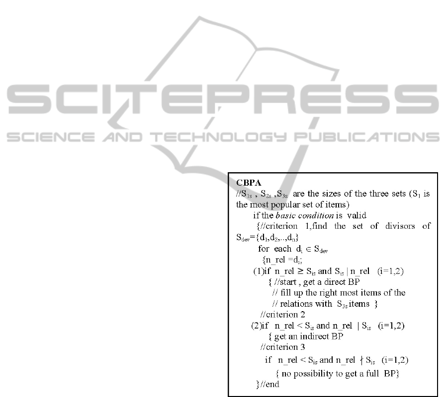
From all the above the pseudo code for the
CBPA is the following:
From all the above, criterion 1 examines the case
of a full direct BP, criterion 2 deals with a full
indirect BP and criterion 3 finds the case of no
possible full BP. Criterion 4 complements the
criteria 1 and 2 for finding equal spacing BP. In case
that CBPA discovers that a full (or optimal) BP can
be achieved the construction of this full BP (CBP)
follows. The parameters for the construction of a BP
such as: n_rel, it_mu
i
for each i set are used for the
ICSOFT 2011 - 6th International Conference on Software and Data Technologies
206

CBP. With the CBP, data are transferred one by one
from the lines of the area_rel into queues and then
the scheduler starts the service directly.
5 THE GDA
The GDA works with creation of the groups using
less number of channels. Economy of channels is
very important factor for large size broadcast cycle.
The grouping is formed so that the AWT
3
is less
than a predefined aver. waiting time for S
3
data. Our
goal is to share the integrated relations to the
channels without changing the RBP. Additionally,
with GDA, the unused channels can be used for
another broadcast data circle dissemination in case
the server works with more than one BP. The
pseudocode of GDA is as follows:
Example 7: Let us consider S
1
= 1, S
2
={2,3,4}, S
3
={5,…,76}with: S
1s
= 1, S
2s
= 3, S
3s
= 72,
pre_av_wt
3
= 40. Here S
3s
>> S
2s
>> S
1s
. Using
CBPA (Lemma 1) the int. divisor of 72 are: 36,
9,8,6,3. The n_rel=36 , it_mu
2
= 36/3 =12. Hence
any item of S
2
will be 12 times in BMP.
We have n_int_rel = 12 (36/3). Because there are 36
relations and the data of S2 are spread along each of
three of them. Analytically the 36 relations are:
(1,2,5,6), (1,3,7,8), (1,4,9,10), (1,2,11,12),
(1,3,13,14), (1,4,15,16), ..,(1,2,71,72), (1,3,73,74),
(1,4,75,76). The 12 integrated relations are:
(1,2,5,6,1,3,7,8,1,4,9,10), (1,2,11,12,1,3,13,14,1,4,
15, 16), ..,(1,2,71,72,1,3,73,74,1,4,75,76).
The int. divisors of 12: 6,4,3. For k=6, m =2 (12/6)
we have the integr. relations: (1,2,5,6),
..,(1,4,39,40)and (1,2,41,42),…,(1,4,75,76). The
AWT3 is: 72. Since 72> 40 a new loop for k=4 is
needed. For k=4, m=3 (12/4) we have the integr.
relations: rel.1: (1,2,5,6),…,(1,4,21,22) , rel.2:
(1,2,23,24), (1,4,39,40), rel.3: (1,2,41,42),.
.,(1,4,57,58), rel.4: (1,2,59,60),..(1,4,75,76).
The AWT
3
= 36< 40. Hence, the minimum
number of channels is: 4 and this can guarantee the
service discrimination.
6 THE HOL-WTG SCHEDULER
We use a Group Round Robin (GRR) scheduler that
provides the service queue order of all the minor
cycles of the sets in a round. The waiting time for an
item i (WT
i
) starts when it becomes HOL until the
beginning of service. When WT
i
becomes greater
than a predefined threshold GRR starts the service of
queue i data. The HOL-WTG (Tsiligaridis et al.,
2007) works like GRR (serves a group of items at a
predefined order) after the weight adjustment (by an
integer multiple of the packet size) and sends the
data to a single or multiple channels.
Lemma 4: The service condition without any waste
of bandwidth is when the bandwidth must be an
integer multiple of the packet size (ps).
Proof: Let us consider as g
i
the size of a minor
circle (i=1,2,3) which is g
i
=ps * n_pac,(1) (where
n_pac is the number of packets, ps is the number of
packets) and bdw = kc * ps (kI) (2). Dividing (1)
by (2) we take g
i
/ bdw = ps * n_pac / kc * ps =
n_pac / kc. If kc=1, then g
i
= bdw * n_pac and the
bdw is used exactly n_pac times in order to service g
i
. If kc ≠ 1, then g
i
= bdw * n_pac /kc . If (n_pac /kc)
= m (mI) then g
i
= bdw * m and no waste of
bandwidth exists. On the other hand if (n_pac /kc) =
m (mN) then there is a surplus of weight (waste)
that services the remainder of data (g
i
mod
bdw).Obviously there is a waste of bandwidth.
GROUPING FOR THE CRITERIA BASED DATA BROADCAST IN WIRELESS MOBILE COMPUTING
207

Example 8: For g
1
(items) = 270b (=30*9), bdw =
60b = 2*30b and (n_pac) / kc = 9/2 = 4.5. The
remainder is 30b (270 mod 60) is serviced by 60b
(bdw). The waste of bandwidth is 30b (=60b-30b)
and loss percentage is: 0.5 (30/60).
Lemma 5: (Bandwidth Adjustment) We consider g
i
(=ps*n_pac) and bandwidth bdw (=kc*ps) having
the packet size (ps) as common factor. In order to
increase the service rate we simply increase kc to m
so that m/n_pac. The variable kc is called increasing
coefficient.
Proof: From g
i
= ps * n_pac, and bdw = kc*ps we
take the ratio: g
i
/ bdw = n_pac / kc =n
1
and n
1
I.
To increase the service ratio we simply find a value
q so that n_pac / (kc + q ) = n
2
and n
2
< n
1
.
Example 9: For g
1
(items) = 300b (=30*10), bdw =
60b=2*30b and (n_pac) / kc = 10/2=5. In order to
reduce the 5 rounds and complete the service to 2,
we increase kc from 2 to 5 (by adding 3). Finally
10/5 =2.
7 SIMULATION
For our simulation, a system with three cooperative
levels is developed: The Application, the Queue and
the List level. In the Application level the items
from the arrays are inserted into the queues. Poisson
arrivals are considered for the mobile users’
requests. The items are separated into three
categories according to their popularity using Zipf
distribution. The Zipf distribution is typically used
to model non uniform access patterns. Three sets are
created; S
1
has the fewest items (most popular), S
2
has the next fewest items (less popular) and S
3
has
the largest number of items (the least popular).
Using the CBPA and then the process of CBP, the
items as encapsulated packets (with ID, queue
number, arrival time, user number) are finally
inserted from the arrays into the correspondent
queues and the HOL-WTG scheduler start their
service. The space of queues is considered as non-
restricted. For our experiments it is considered that
the server has additional bandwidth (weight)
available in order to be able to adjust the weights.
Four scenaria have been developed:
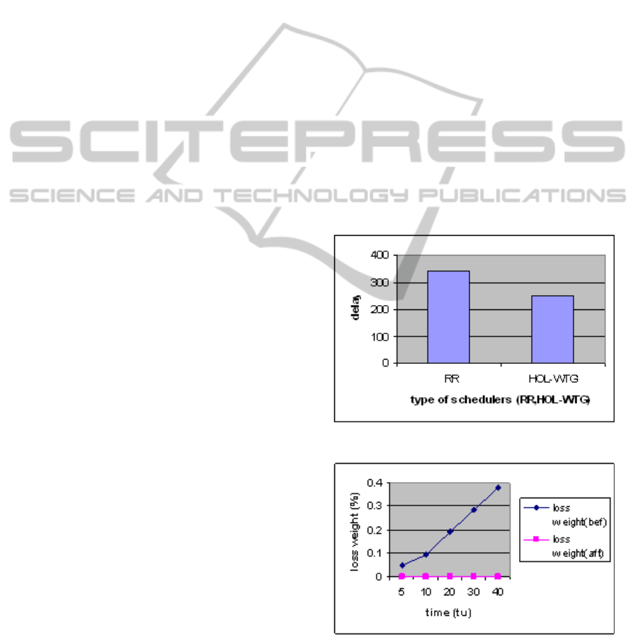
Scenario 1: The service time of a RR scheduler and
HOL-AW scheduler are compared in a broadcast
program with the three categories of sets. The HOL-
AW scheduler (Fig. 1) reduces the service time by
adjusting (increasing) the weight provided better
results (450 tu instead of 630 tu).
Scenario 2: In Fig. 2 there is an increasing waste of
weight before the use of the HOL-WTG scheduler.
Scenario 3: In Fig. 3, data in various sizes with
equal spacing (RBP) from S
1
and S
2
sets, and flat
(for all the sets) with long broadcast cycle size are
depicted. For the data with equal spacing the AWT
is less than the one of the flat data. It is considered a
single channel service. We will also take the same
results of the RBP for the users interested in data of
S
1
, S
2
if more channels were used (as in example 6).
Scenario 4: Three set of data are used and three
cases (each one for each set) are developed starting
from left to right in Fig. 4. All of them have the
same S
1
data. The second set has more data
(relations) of S
3
and the same size of S
2
data
(relations). Because of this, in the second case four
channels are used instead of three in order to provide
the same AWT
3
. The number of channels are
selected according to GDA considering pre_av_wt
3
= 40sec. The third set has more data on S3 and less
data on S2 comparing with the data of the second
set. Because of this there is an increase of AWT
3
(18
sec comparing with 16sec) and a decrease of AWT
2
(from 8sec to 6sec).
Figure 1: HOL-AW vs RR for delay.
Figure 2: The waste of weight before and after HOL-
WTG.
ICSOFT 2011 - 6th International Conference on Software and Data Technologies
208

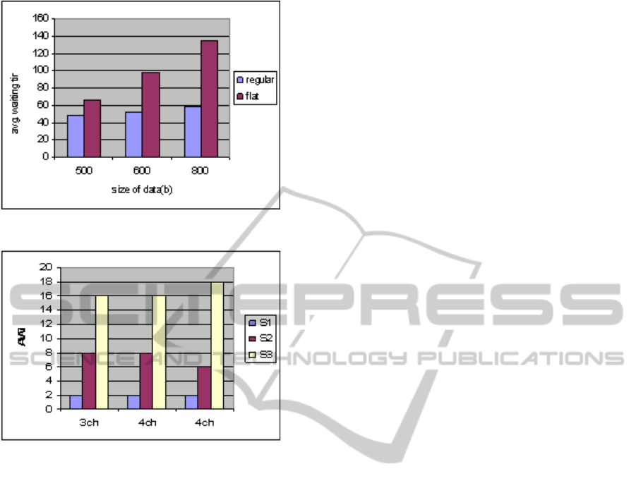
Figure 3: The AWT for regular and flat data.
Figure 4: AWT with GDA grouping.
8 CONCLUSIONS
A new method for regular data broadcasting, based
on criteria, has been developed. The proposed
method of designing broadcast plans with the ability
of HOL-WTG scheduler to reduce the service time
of users’ data, according to the desired waiting time,
can provide new opportunities for the scale-up
servers. It can enhance their self-sufficiency, self-
monitoring. Such servers may address quality of
service, and other issues with minimal human
intervention.
REFERENCES
A. Bertossi. A, M. Pinotti, M., S. Ramaprasad, S., Rizzi,
R., M. Shashanka, M., 2004. “Optimal multi-channel
data allocation with flat broadcast per channel”,
Proceedings of IPDS’04, pp.18-27.
Acharya, S., Franklin, M., Zdonik, S., Alonso, R.,
1995.“Broadcast disks: Data management for
asymmetric communications environments“,
Proceedings of the ACM SIGMOD Intern. Conf. on
Management of Data, San Jose, May 1995, pp.199-
210.
Sumari, P., Darus, R., Kamarulhaili, H., 2003. “Data
Organization for Broadcasting in Mobile
Computing “, Proceedings of IEEE Int. Conf. on
Geometric Modeling and Graphics(GMAG’03).
Bowen, T., Gopal, G., Herman, G., Hickey, T., 1992. “The
datacycle architecture”, CACM35(12) , pp71-81.
Acharya, S., Franklin, M., Zdonik, S., 1996. “Perefetching
from a Booadcast Disk”, Proceedings of Inter. Conf.
on Data Engineering, New Orleans, LA. Kenyon, C.,
Schabanel, N., Young, N., 2000. “Polynomial-Time
Approximation scheme for data broadcast”,
Proceedings of 32 ACM Sumposium on Theory of
Computing, Portland, OR, May 21-23, pp.659- 666.
Bar-Noy, A. Ladner, R., 2003. “Windows Scheduling
Problems for Broadcast Systems”, SIAM Journal on
Computing”, V.32, Isssue: 4, 2003, pp.1091-1113.
Tsiligaridis, J., R. Acharya, R., 2007. “An Adaptive Data
Broadcasting Model in Mobile Information Systems”,
6
th
International Conference on Computer Information
Systems and Industrial Management Applications,
CISIM, pp.203-208.
GROUPING FOR THE CRITERIA BASED DATA BROADCAST IN WIRELESS MOBILE COMPUTING
209