UF-EVOLVE - UNCERTAIN FREQUENT PATTERN MINING
Shu Wang and Vincent Ng
Department of Computing, The Hong Kong Polytechnic University, Hung Hom, Kowloon, Hong Kong
Keywords: Uncertain frequent pattern mining, Tree, Shuffling and merging.
Abstract: Many frequent-pattern mining algorithms were designed to handle precise data, such as the FP-tree structure
and the FP-growth algorithm. In data mining research, attention has been turned to mining frequent patterns
in uncertain data recently. We want frequent-pattern mining algorithms for handling uncertain data. A
common way to represent the uncertainty of a data item in record databases is to associate it with an
existential probability. In this paper, we propose a novel uncertain-frequent-pattern discover structure, the
mUF-tree, for storing summarized and uncertain information about frequent patterns. With the mUF-tree,
the UF-Evolve algorithm can utilize the shuffling and merging techniques to generate iterative versions of
it. Our main purpose is to discover new uncertain frequent patterns from iterative versions of the mUF-tree.
Our preliminary performance study shows that the UF-Evolve algorithm is efficient and scalable for mining
additional uncertain frequent patterns with different sizes of uncertain databases.
1 INTRODUCTION
Data uncertainty is often found in real-world
applications because of measurement inaccuracy,
sampling discrepancy, outdated data sources, or
other errors. One type of data uncertainty is
existential uncertainty. In existential uncertainty,
there are applications in which it is uncertain about
the presence or absence of some items or events. For
example, we may highly suspect, while cannot
guarantee, that a patient suffers from an illness based
on a few symptoms. The uncertainty of such
suspicion can be expressed in terms of existential
probability. If R
i
represents a patient record, then
each item within R
i
represents an illness and is
associated with an existential probability expressing
the likelihood of the patient suffering from that
illness in R
i
. As an example, in R
i
, the patient can
have an 80% likelihood of suffering from fever, and
a 60% likelihood of suffering from H1N1.
Han et al. (Han, 2004) proposed the FP-tree
structure, which is an extended prefix-tree structure
for storing compressed, crucial information about
frequent patterns, and developed an efficient FP-
growth algorithm. In our work, we extend the FP-
tree for mining uncertain data. The key contributions
are (i) the development of the mUF-tree structure to
summarize the content of records consisting of
uncertain data, and (ii) the idea of shuffling and
merging nodes of mUF-tree, whose difference is
small, to derive more uncertain frequent patterns by
the UF-Evolve algorithm.
The remainder of the paper is organized as
follows. Section 2 gives a literature review and
Section 3 gives the problem statement. Section 4
introduces the mUF-tree and its construction
algorithm. Next, Section 5 discusses an mUF-tree-
based uncertain-frequent-pattern mining algorithm,
the UF-Evolve algorithm, and Section 6 presents our
performance study. Finally, Section 7 concludes our
work.
2 LITERATURE REVIEW
For uncertain data representation, Antova et al.
(Antova, 2007) proposed U-relations, a succinct and
purely relational representation system for uncertain
databases. U-relations support attribute-level
uncertainty using vertical partitioning. When
considering positive relational algebra extended by
an operation for computing possible answers, a
query on the logical level can be translated into, and
evaluated as, a single relational algebra query on the
U-relation representation. The approach takes full
advantage of query evaluation and optimization
techniques on vertical partitions. Chui et al. (Chui,
2007) proposed an algorithm called U-Apriori. They
74
Wang S. and Ng V..
UF-EVOLVE - UNCERTAIN FREQUENT PATTERN MINING.
DOI: 10.5220/0003499400740084
In Proceedings of the 13th International Conference on Enterprise Information Systems (ICEIS-2011), pages 74-84
ISBN: 978-989-8425-53-9
Copyright
c
 2011 SCITEPRESS (Science and Technology Publications, Lda.)

also introduced a trimming strategy to reduce the
number of candidates that need to be counted based
on the Apriori approach. The Apriori heuristic
achieves good performance gained by (possibly
significantly) reducing the size of candidate sets.
However, in situations with a large number of
frequent patterns, long patterns, or low minimum
support thresholds, an Apriori-like algorithm may
suffer from the following two nontrivial issues: it is
costly to handle a huge number of candidate sets;
and it is tedious to repeatedly scan the database and
check a large set of candidates by pattern matching,
which is especially true for mining long patterns.
Han et al. (Han, 2004) proposed the FP-tree
structure and the FP-growth algorithm for efficiently
mining frequent patterns without generation of
candidate itemsets for precise data. It consists of two
phases. The first phase focuses on constructing the
FP-tree from the database, and the second phase
focuses on applying FP-growth to derive frequent
patterns from the FP-tree. Each node in the FP-tree
consists of three attributes, item-name, count and
node-link. In the FP-tree, each entry in the header
table consists of two fields: (1) item-name, and (2)
head of node-links (a pointer pointing to the first
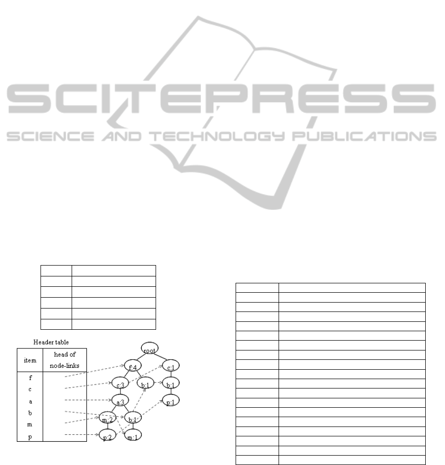
node in the FP-tree carrying the item-name). Below,
an example is used to illustrate the uses of the FP-
tree. Suppose there is a precise transaction database
as shown in Table 1, and the minimum support
threshold is 3. The FP-tree together with the
associated node-links are shown in Figure 1.
Table 1: A precise transaction database.
TID Items
1 f, a, c, d, g, i, m, p
2 a, b, c, f, l, m, o
3 b, f, h, j, o
4 b, c, k, s, p
5 a, f, c, e, l, p, m, n
Figure 1: The FP-tree for data in Table 1.
Leung et al. (Leung, 2007 and 2008) proposed
the UF-tree structure, a different tree structure than
the FP-tree for capturing the content of transactions
consisting of uncertain data, and the UF-growth
algorithm, a mining algorithm for finding frequent
patterns from the UF-tree. Each node in the UF-tree
stores item, expected support and occurrence (i.e.
the number of transactions containing such an item).
UF-growth computes expected support of itemsets
and finds frequent patterns from the UF-tree. The
expected support of an itemset in a transaction is the
expected probability (over all “possible worlds”) of
coexistence of all the items in the itemset. The
expected support of an itemset in a database is the
sum of the expected probability of the itemset over
all transactions. This calculation incurs much
information loss.
3 PROBLEM STATEMENT
Here, in this section, we give some definitions of
uncertain data before introducing our target problem.
First, we define what an uncertain record and an
uncertain database are.
Definition 1. Uncertain Record (R). Let I = {a
1
, a
2
,
…, a
k
} be a set of items. An uncertain record R =
{(a
1
:p
1
), (a
2
:p
2
), …, (a
m
:p
m
)}, where (a
i
∈ I)
∧
(a
i
appears once with p
i
as the probability indicating its
existence).
Definition 2. Uncertain Database (UDB). An
uncertain database UDB consists of multiple
uncertain records, i.e. UDB = <R
1
, R
2
, …, R
n
>.
An example uncertain database is shown in Table 2.
Table 2: An uncertain database.
Record ID Item:probability pairs
1 (a:0.2), (f:0.8), (g:0.1), (d:0.3), (c:0.2)
2 (a:0.2), (d:0.3), (c:0.2), (f:0.8)
3 (b:0.3), (f:0.8), (a:0.2)
4 (a:0.4), (c:0.7), (d:0.6), (f:0.8)
5 (f:0.8)
6 (a:0.7), (c:0.4), (b:0.5)
7 (a:0.7)
8 (f:0.8), (a:0.4), (c:0.7), (d:0.6)
9 (b:0.5), (a:0.7), (c:0.4)
10 (d:0.4), (e:0.5), (f:1.0), (a:0.1)
11 (e:0.6), (c:0.3), (d:0.5), (a:0.1), (f:1.0)
12 (a:0.1), (f:1.0), (c:0.3), (d:0.5)
13 (a:0.1), (f:1.0)
14 (f:1.0)
15 (d:0.4), (c:0.4), (b:0.2)
16 (b:0.2)
17 (b:0.2), (f:0.6)
18 (b:0.2)
In an uncertain database, it is often that an item
with a probability appears in a record while the same
item with another probability appears in another
UF-EVOLVE - UNCERTAIN FREQUENT PATTERN MINING
75

record. For example, in Table 2, (d:0.4) appears in
the 10
th
record while (d:0.5) appears in the 11
th
record. Given a predefined minimum support
threshold, an item with a specific probability may
not have sufficient support (i.e. the number of
records containing it in UDB) to be a frequent
pattern.
In order to improve the chance of having more
and longer frequent patterns, one can consider to
merge the same items with only small differences in
their various probabilities for satisfying the support.
For example, we can merge (d:0.4) and (d:0.5) as d
with a probability range [0.4-0.5]. Hence, for a
group of item:probability pairs in which all items are
the same, we can use (lowerbound-upperbound) to
represent the spread of probabilities for the item.
Once the item:probability pairs are grouped, more
general frequent patterns can be found.
With the above arrangement, we define what a
maximum merging threshold and an uncertain
frequent pattern are.
Definition 3. Maximum Merging Threshold (
γ
).
A maximum merging threshold
γ
is used to
determine whether two item:probability pairs can be
merged. Assume that an item with a probability (a:p
1
)
appears in a record while the same item with another
probability (a:p
2
) appears in another record. If abs(p
1
– p
2
)
γ
≤ , then (a:p
1
) and (a:p
2
) can be merged as
(a:[l-u]), where (l = min(p
1
, p
2
)) ∧ (u = max(p
1
,
p
2
)). Here, (a:[l-u]) denotes the item with its
(lowerbound-upperbound).
Definition 4. Uncertain Frequent Pattern (UFP).
Let an item with its (lowerbound-upperbound) be
denoted as (a:[l-u]). An uncertain frequent pattern
UFP is represented as (a
1
:[l
1
-u
1
])(a
2
:[l
2
-u
2
])…(a
k
:[l
k
-
u
k
]):s, where (s is the support for UFP)
∧
(s ≥ a
predefined minimum support threshold). A record R
contains an UFP if for each (a
i
:[l
i
-u
i
])
∈
UFP,
∃
(a
j
:p
j
) ∈ R, such that (a
i
= a
j
) ∧ (l
i
≤ p
j
≤ u
i
).
Given an uncertain database, a minimum support
threshold and a maximum merging threshold, we are
interested in mining a possible set of uncertain
frequent patterns. Our approach is to solve the
problem in two phases.
• In the first phase, an mUF-tree is constructed for
storing summarized and uncertain information about
frequent patterns.
• In the second phase, the UF-Evolve algorithm,
which utilizes the shuffling and merging techniques
to generate iterative versions of the mUF-tree, is
applied for discovering new uncertain frequent
patterns.
4 MUF-TREE: DESIGN AND
CONSTRUCTION
Given an uncertain database, we propose to use an
mUF-tree to store summarized and uncertain
information about frequent patterns. An mUF-tree
with its header table is shown in Figure 2.
Figure 2: mUF-tree.
Definition 5. Uncertain Frequent Pattern Tree
(mUF-tree). An mUF-tree has the following
characteristics.
1. An mUF-tree has a virtual root. Each node in the
mUF-tree consists of five attributes, item,
lowerbound, upperbound, frequency and node-link.
Lowerbound and upperbound register the spread of
probabilities of the corresponding item. To facilitate
tree traversal, nodes with the same
item:(lowerbound-upperbound) are linked in
sequence via node-links. In Figure 2, a
i
:[l
i
-u
i
]:f
i
in
each node N
i
represents item:(lowerbound-
upperbound):frequency.
2. In the mUF-tree, each entry in the header table
consists of four fields: (1) item, (2) lowerbound-
upperbound, (3) support (the cumulative frequency
of the item:(lowerbound-upperbound) in the mUF-
tree), and (4) head of node-links (a pointer pointing
to the first node in the mUF-tree carrying the
item:(lowerbound-upperbound)).
3. In the header table, item:(lowerbound-
upperbound) pairs are in the descending order of
supports.
The UF-Construct algorithm is used to construct an
mUF-tree from an uncertain database, and its output
is the initial mUF-tree. Unlike the FP-tree
construction algorithm, UF-Construct scans the
database without specifying a minimum support
threshold. With this change, the mUF-tree built
contains all information. Compared with FP-tree, the
mUF-tree stores uncertain information about items,
and maintains the structure to be further modified
ICEIS 2011 - 13th International Conference on Enterprise Information Systems
76

for discovering more uncertain frequent patterns.
Figure 3 shows the steps of the UF-Construct
algorithm.
UF-Construct algorithm.
Input: A UDB.
Output: An mUF-tree T.
Procedure UF-Construct(UDB)
(1)
(2)
(3)
(4)
(5)
(6)
(7)
(8)
(9)
(10)
(11)
(12)
(13)
(14)
(15)
scan UDB once and collect a_set = the set of items
with their respective supports in descending order;
create T with a root;
for each record R in UDB do {
R’ = the item:probability pairs in R with items
putting in the same order as in a_set;
r = root(T);
for i = 1 to length(R’) do {
(a
i
:p
i
) = the i
th
item:probability pair of R’;
find N
c
= child(r), where (N
c
.a
c
= a
i
) ∧ (N
c
.l
c
=
p
i
);
if
∃ N
c
then N
c
.f
c
++;
else {
create node N
c
with (N
c
.a
c
= a
i
) ∧
(N
c
.l
c
= N
c
.u
c
= p
i
)
∧
(N
c
.f
c
= 1);
insert N
c
as the rightmost child of r;
}
update header table and node-links within T;
r = N
c
;
}
}
return T;
Figure 3: UF-Construct.
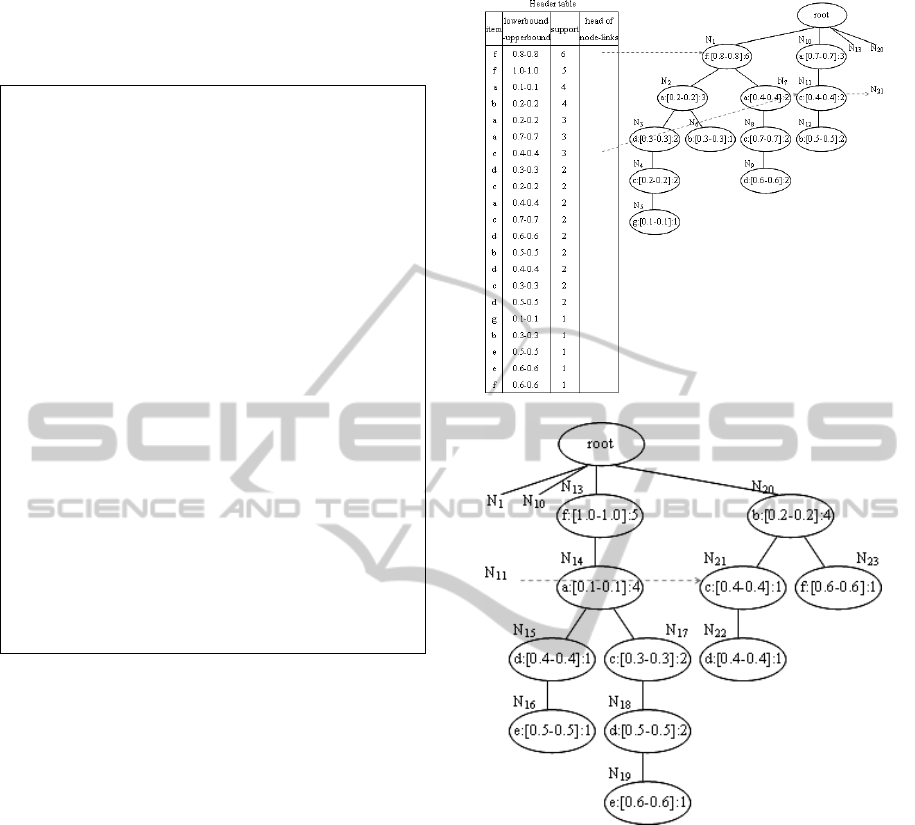
With the records in Table 2, the mUF-tree
together with the associated node-links are shown in
Figure 4. Since the constructed mUF-tree is large,
we split it into two parts. Figure 4(a) shows the
header table with the left half of the mUF-tree, and
Figure 4(b) shows the right half of the mUF-tree.
For the ease of understanding, we only show several
node-links.
5 DISCOVERING NEW
UNCERTAIN FREQUENT
PATTERNS
If we want to use the FP-growth algorithm to mine
frequent patterns with mUF-tree(right) in Figure
4(b), we can consider a
i
:[l
i
-u
i
] as an item.
Then FP-growth will discover a set of frequent
patterns {(b:[0.2-0.2]):4, (a:[0.1-0.1]):4, (f:[1.0-
1.0])(a:[0.1-0.1]):4, (f:[1.0-1.0]):5} with the
minimum support threshold be 3.
In
an mUF-tree, it is often that an item with a
(a) mUF-tree(left).
(b) mUF-tree(right).
Figure 4: The mUF-tree for data in Table 2.
(lowerbound-upperbound) appears in a node while
the same item with another (lowerbound-
upperbound) appears in another node. For example,
in Figure 4(b), d:[0.4-0.4] appears in N
15
while
d:[0.5-0.5] appears in N
18
. One can consider to
merge the same items with only small differences in
their various (lowerbound-upperbound) for
satisfying the support. For example, we can merge
d:[0.4-0.4] and d:[0.5-0.5] as d:[0.4-0.5]. Hence, for
a group of item: (lowerbound-upperbound) pairs of
the same item, we can use a combined (lowerbound-
upperbound) to represent it. Once the
item:(lowerbound-upperbound) pairs are grouped,
more general frequent patterns can be found.
UF-EVOLVE - UNCERTAIN FREQUENT PATTERN MINING
77

Hence, we are proposing to further discover new
uncertain frequent patterns by utilizing shuffling and
merging of the mUF-tree. Nodes can be merged to
evolve into another mUF-tree for further pattern
mining. The steps can be repeated until merging is
not possible.
5.1 Preliminary Definitions
For the ease of future discussion, we have further
definitions before presenting the algorithms.
Definition 6. Within Range. Given a maximum
merging threshold
γ
, we define two nodes N
b
and
N
c
are within range if (N
b
.a
b
= N
c
.a
c
) ∧ (abs(N
b
.u
b
– N
c
.l
c
)
γ
≤ ) ∧ (abs(N
c
.u
c
– N
b
.l
b
)
γ
≤ ).
In Figure 4(b), given a maximum merging threshold
0.3, then N
15
and N
18
are within range, as well as N
16
and N
19
are within range.
Definition 7. Common Items (CI). Given a pair of
paths PB = <N
b1
N
b2
…N
bk
> and PC =
<N
c1
N
c2
…N
cm
>, we define CI(PB, PC) = {a
1
, a
2
, …,
a
n
} as a sequence of ordered items, where (n
≤
k)
∧
(n ≤ m)
∧
(
∀
i
∈
{1, 2, …, n}, there is a node
in PB and a node in PC, such that these two nodes
contain a
i
and are within range).
In Figure 4(b), given a pair of paths PB = <N
15
N
16
>
and PC = <N
17
N
18
N
19
>, then CI(PB, PC) = {d, e}.
We want to merge the nodes corresponding to
common items in the two paths. However, it is
difficult to merge N
15
with N
18
and N
16
with N
19
directly. We need to shuffle these nodes to be in the
same order. Here, we define the Maximum
Attainable Peak (MAP) of a node in a path first.
Definition 8. Maximum Attainable Peak (MAP).
Given a_set = {a
11
, a
12
, …, a
1k
} as a sequence of
ordered items, and a path PB = <N
21
N
22
…N
2m
>,
where the items in a_set is a subset of the items in
PB. We take out each item a
1i
in a_set sequentially
and trace along PB. If the position of a
1i
in PB is not
as in a_set, the node N
2j
containing a
1i
will be
shuffled upward until the position of a
1i
in PB is as
in a_set. The final position is called the MAP of N
2j
in PB.
Now, we are ready to describe two cases for
shuffling the node N
2j
with its parent node N
q
.
• Case 1: N
2j
.f
2j
= N
q
.f
q
. Swap N
2j
and N
q
.
• Case 2: N
2j
.f
2j
< N
q
.f
q
. Create a new node, N
r
,
with the same property of N
q
except N
r
.f
r
= N
q
.f
q
–
N
2j
.f
2j
. Make N
r
as another child of the parent of N
q
.
Set N
q
.f
q
= N
2j
.f
2j
. Update the header table and node-
links within the mUF-tree, and then follow the
handling of Case 1 for N
2j
and N
q
.
The node N
2j
will be shuffled until it reaches its
MAP in PB.
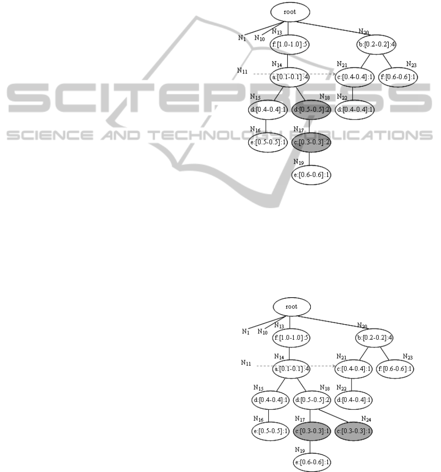
In Figure 4(b), given a_set = {d, e}, then the
MAP of N
18
in the path <N
17
N
18
N
19
> is the 1
st
position. We shuffle N
18
with N
17
, which follows
Case 1. mUF-tree(right) evolves into mUF-
tree(right)
2
, as shown in Figure 5.
Figure 5: mUF-tree(right)
2
.
After shuffling N
18
to its MAP, the MAP of N
19
in the updated path <N
18
N
17
N
19
> is the 2
nd
position.
We shuffle N
19
with N
17
, which follows Case 2. We
create a new node N
24
and modify N
17
, which
evolves into mUF-tree(right)
3
, as shown in Figure 6.
Then we shuffle N
19
with N
17
, which evolves into
mUF-tree(right)
4
, as shown in Figure 7.
Figure 6: mUF-tree(right)
3
.
ICEIS 2011 - 13th International Conference on Enterprise Information Systems
78

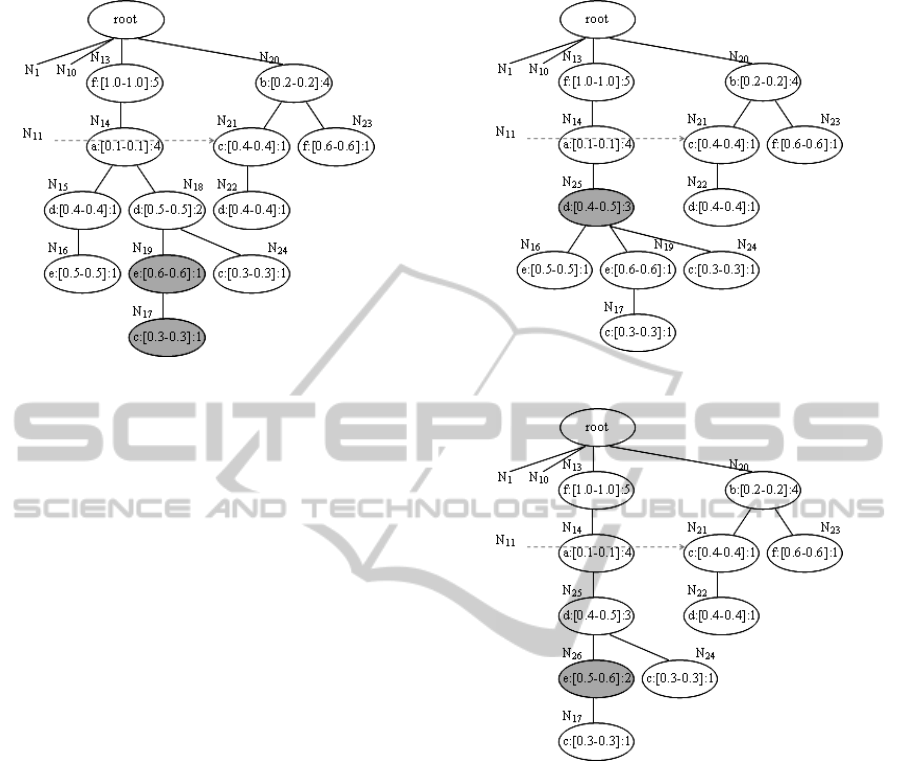
Figure 7: mUF-tree(right)
4
.
After shuffling, the nodes corresponding to
common items are above the other nodes in the two
paths. It is much easier to merge N
15
with N
18
and
N
16
with N
19
.
Next, we define the merging criteria, which
determine how two candidate nodes can be merged
to a new node.
Definition 9. Merging Criteria. If two nodes N
b
and N
c
are within range, they can be merged as a
new node N
q
, where (N
q
.a
q
= N
b
.a
b
) ∧ (N
q
.l
q
=
min(N
b
.l
b
, N
c
.l
c
)) ∧ (N
q
.u
q
= max(N
b
.u
b
, N
c
.u
c
))
∧
(N
q
.f
q
= N
b
.f
b
+ N
c
.f
c
).
We merge N
15
with N
18
as a new node N
25
,
which evolves into mUF-tree(right)
5
, as shown in
Figure 8. And then we merge N
16
with N
19
as a new
node N
26
, which evolves into mUF-tree(right)
6
, as
shown in Figure 9.
Definition 10. Overlap. Given a path PB,
overlap(PB) is true if PB shares common nodes with
any other path in the mUF-tree.
In Figure 4(b), given PB = <N
13
N
14
N
15
N
16
>, PC
= <N
13
N
14
N
17
N
18
N
19
> and PD = <N
17
N
18
N
19
>, then
overlap(PB) since PB shares N
13
and N
14
with PC,
and !overlap(PD) since PD does not share common
nodes with any other path.
Definition 11. Above. Given a_set = {a
11
, a
12
, …,
a
1k
} and a path PB = <N
21
N
22
…N
2m
>, above(a_set ,
PB) is true if (k
≤ m) ∧ (
∀
i ∈ {1, 2, …, k}, a
1i
=
N
2i
.a
2i
).
In Figure 4(b), given a_set = {d, e}, PB =
<N
15
N
16
> and PC = <N
17
N
18
N
19
>, then above(a_set,
PB) since d and e are above other items in PB, and
!above(a_set, PC) since d and e are not above other
items in PC.
Figure 8: mUF-tree(right)
5
.
Figure 9: mUF-tree(right)
6
.
There can be five cases for shuffling a pair of
paths PB and PC. In Case 1, both PB and PC do not
share common nodes with any other path in the
mUF-tree. Therefore, PB and PC can be shuffled
without influencing others. In Case 2, PB does not
share common nodes with any other path, but PC
does. However, in PC, the nodes with common items
are above other nodes. Therefore, we do not need to
shuffle PC. Case 3 is similar to Case 2 with the
information in PB and PC inter-changed. In Case 4,
both PB and PC share common nodes with other
paths, but with nodes having common items above
other nodes. Therefore, neither PB nor PC needs to
be shuffled. For all the four cases, PB and PC can be
merged after shuffling if necessary.
All other conditions beside the above are
considered as Case 0. In Case 0, shuffling is not
allowed. Since shuffling in the two paths may induce
much effort in re-structuring of the whole mUF-tree.
UF-EVOLVE - UNCERTAIN FREQUENT PATTERN MINING
79

Definition 12. Shuffle Case (SC). Given a pair of
paths PB and PC, and a_set = CI(PB, PC), there are
five shuffle cases.
• SC(PB, PC) = 1 if !overlap(PB)
∧ !overlap(PC).
• SC(PB, PC) = 2 if !overlap(PB)
∧ overlap(PC)
∧ above(a_set, PC).
• SC(PB, PC) = 3 if overlap(PB)
∧ above(a_set,
PB) ∧ !overlap(PC).
• SC(PB, PC) = 4 if overlap(PB)
∧ above(a_set,
PB) ∧ overlap(PC) ∧ above(a_set, PC).
• SC(PB, PC) = 0 for other conditions.
For the ease of understanding, the shuffle cases are
shown in Table 3.
Table 3: Shuffle cases.
SC(PB, PC) !overlap(PC)
overlap(PC)
∧
above(a_set, PC)
!overlap(PB) 1 2
overlap(PB) ∧
above(a_set, PB)
3 4
Take the mUF-tree in Figure 4 as an example.
Given a maximum merging threshold 0.3, then the
shuffle cases with the corresponding path pairs are
shown in Table 4.
Table 4: Shuffle cases with corresponding path pairs.
PB PC
CI(PB,
PC)
SC(PB,
PC)
<N
15
N
16
> <N
17
N
18
N
19
> {d, e} 1
<N
10
N
11
N
12
> <N
20
N
21
N
22
> {b, c} 2
<N
2
N
3
N
4
N
5
> <N
7
N
8
N
9
> {a, d} 3
<N
1
N
2
N
3
N
4
N
5
> <N
13
N
14
N
15
N
16
> {f, a, d} 4
<N
10
N
11
N
12
> <N
13
N
14
N
17
N
18
N
19
> {c} 0
<N
1
N
7
N
8
N
9
> <N
20
N
23
> {f} 0
<N
1
N
2
N
6
> <N
10
N
11
N
12
> {b} 0
<N
1
N
2
N
6
> <N
20
N
23
> {b, f} 0
<N
1
N
7
N
8
N
9
> <N
20
N
21
N
22
> {c, d} 0
Definition 13. Common Ancestor Path (CAP).
Given a pair of paths PB = <N
b1
N
b2
…N
bk
> and PC =
<N
c1
N
c2
…N
cm
>, we define CAP(PB, PC) =
<N
b1
N
b2
…N
bn
>, where (n
≤
k) ∧ (n ≤ m)
∧
(
∀
i
∈
{1, 2, …, n}, N
bi
and N
ci
are the same node).
In Figure 4(b), given a pair of paths PB =
<N
13
N
14
N
15
N
16
> and PC = <N
13
N
14
N
17
N
18
N
19
>, then
CAP(PB, PC) = <N
13
N
14
>.
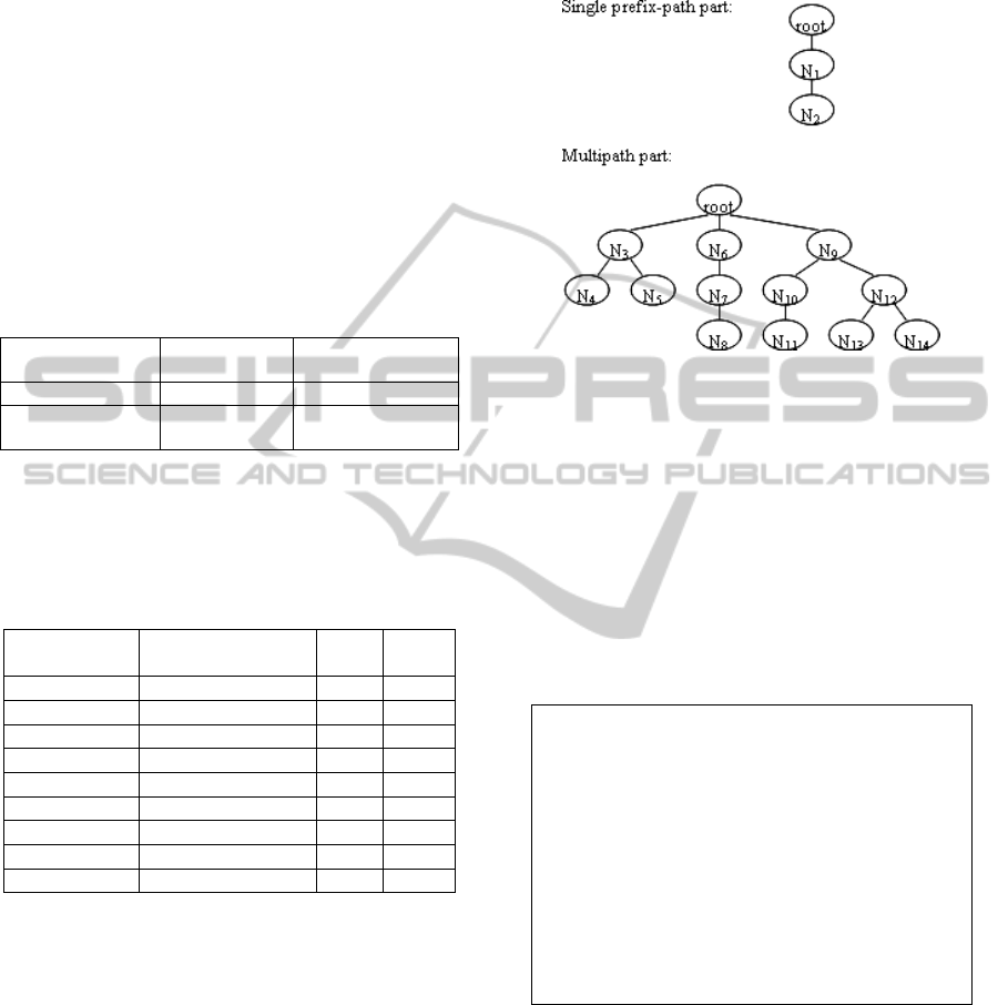
Definition 14. Single Prefix-Path Part and
Multipath Part. The single prefix-path part of an
mUF-tree consists of a single path from the root to
N
k
, the first node containing more than one child.
The multipath part of an mUF-tree consists of the
descendants of N
k
, with a virtual root connecting to
the children of N
k
as the parent.
For the mUF-tree shown in Figure 2, the single
prefix-path part and the multipath part are shown in
Figure 10.
Figure 10: Single prefix-path part and multipath part of
mUF-tree.
5.2 The UF-Evolve Algorithm
With the aforementioned definitions, we present the
UF-Evolve algorithm for mining frequent patterns in
an uncertain database by using an mUF-tree. The
algorithm integrates the UF-Mine algorithm for
finding out the possible frequent patterns and the
UF-Shuffle algorithm for moving and merging the
nodes in the mUF-tree iteratively. Figure 11 shows
the steps of the UF-Evolve algorithm.
UF-Evolve algorithm.
Input: An mUF-tree T, a minimum support threshold
σ
, and a maximum merging threshold
γ
.
Output: A set of uncertain frequent patterns.
Procedure UF-Evolve(T,
σ
,
γ
)
(1)
FPS =
φ
; // Frequent pattern set
(2)
(3)
(4)
do {
FPS = FPS
∪
UF-Mine(T, null,
σ
);
T = UF-Shuffle(T,
γ
);
(5)
(6)
} while T has been modified;
return FPS;
Figure 11: UF-Evolve.
In line (17) of Figure 12, (FPS(P) × FPS(Q))
means concatenating each frequent pattern FP
i
in
FPS(P) with each frequent pattern FP
j
in FPS(Q),
with support equal to FP
j
.support.
In order to illustrate how the different algorithms
work, we will use a running example with mUF-
tree(right) in Figure 4(b). Suppose the minimum
support threshold is 3, and the maximum merging
threshold
is 0.3. UF-Evolve calls UF-Mine, and UF-
ICEIS 2011 - 13th International Conference on Enterprise Information Systems
80

UF-Mine algorithm.
Input: An mUF-tree T, an uncertain frequent pattern
α
=
(a
1
:[l
1
-u
1
])(a
2
:[l
2
-u
2
])…(a
k
:[l
k
-u
k
]):s, and a minimum
support threshold
σ
.
Output: A set of uncertain frequent patterns.
Procedure UF-Mine(T,
α
,
σ
)
(1)
(2)
P = the single prefix-path part of T;
Q = the multipath part of T;
(3)
FPS(P) =
φ
; // Frequent pattern set in P
(4)
FPS(Q) =
φ
; // Frequent pattern set in Q
(5)
for each pattern
β
formed from P where all
nodes in
β
have sufficient support do {
(6)
β
.support = minimum support of nodes in
β
;
(7)
append
α
to the end of
β
;
(8)
FPS(P) = FPS(P)
∪
β
;
(9)
}
for each (a
i
:[l
i
-u
i
]) in Q with sufficient support do {
(10)
β
= (a
i
:[l
i
-u
i
]);
(11)
β
.support = (a
i
:[l
i
-u
i
]).support;
(12)
append
α
to the end of
β
;
(13)
FPS(Q) = FPS(Q)
β
∪ ;
(14) find cond_tree from Q constructed with the
conditional pattern-base of
β
;
// Conditional mUF-tree of
β
(15)
(16)
if
∃ cond_tree then
FPS(Q) = FPS(Q)
∪
UF-Mine(cond_tree,
β
,
σ
);
}
(17)
return FPS(P)
∪ FPS(Q) ∪
(FPS(P)
× FPS(Q));
Figure 12: UF-Mine.
Mine returns a set of uncertain frequent patterns,
which is {(b:[0.2-0.2]):4, (a:[0.1-0.1]):4, (f:[1.0-
1.0])(a:[0.1-0.1]):4, (f:[1.0-1.0]):5}.
The core algorithm is the UF-Shuffle algorithm,
which is shown in Figure 13. Each time it is called
by UF-Evolve, it collects the set of paths under the
root and finds the most suitable pair of paths to
shuffle and merge.
There can be different versions of the UF-Shuffle
algorithm. Figure 14 shows UF-Shuffle_2, which is
a variant of UF-Shuffle. Each time it is called by
UF-Evolve, it collects the set of paths under the root
and tries to shuffle and merge each pair of paths. If a
pair of paths are shuffled and merged, they will be
removed from the set of paths since they have been
modified and no longer exist.
After
shuffling, candidate nodes can then be
UF-Shuffle algorithm.
Input: An mUF-tree T, and a maximum merging threshold
γ
.
Output: A shuffled mUF-tree T.
Procedure UF-Shuffle(T,
γ
)
(1)
(2)
(3)
(4)
(5)
(6)
(7)
(8)
(9)
(10)
(11)
(12)
(13)
(14)
(15)
scan T once and collect P_set = the set of paths under
root(T);
for each pair of paths PB and PC in P_set do {
P = CAP(PB, PC);
PB = PB excludes P;
PC = PC excludes P;
get CI(PB, PC) and SC(PB, PC);
}
suppose (PB’, PC’) is a pair of paths that (has maximum
length(CI(PB, PC)))
∧
(length(CI(PB’, PC’)) > 0)
∧
(SC(PB’, PC’) > 0);
if
∃
(PB’, PC’) then {
switch SC(PB’, PC’) {
case 1: shuffle the nodes corresponding to CI(PB’,
PC’) to their MAP in PB’ and PC’;
case 2: shuffle the nodes corresponding to CI(PB’,
PC’) to their MAP in PB’;
case 3: shuffle the nodes corresponding to CI(PB’,
PC’) to their MAP in PC’;
case 4: do nothing;
}
T = UF-Merge(T, PB’, PC’,
length(CI(PB’, PC’)));
}
return T;
Figure 13: UF-Shuffle.
Procedure UF-Shuffle_2(T,
γ
)
(1)
(2)
(3)
(4)
(5)
(6)
(7)
(8)
(9)
(10)
(11)
(12)
(13)
(14)
scan T once and collect P_set = the set of paths under
root(T);
for each pair of paths PB and PC in P_set do {
P = CAP(PB, PC);
PB = PB excludes P;
PC = PC excludes P;
if (length(CI(PB, PC)) > 0)
∧
(SC(PB, PC) > 0) then {
switch SC(PB, PC) {
case 1: shuffle the nodes corresponding to CI(PB,
PC) to their MAP in PB and PC;
case 2: shuffle the nodes corresponding to CI(PB,
PC) to their MAP in PB;
case 3: shuffle the nodes corresponding to CI(PB,
PC) to their MAP in PC;
case 4: do nothing;
}
T = UF-Merge(T, PB, PC,
length(CI(PB, PC)));
remove PB and PC from P_set;
// Updates will be used in loop at line (2)
}
}
return T;
Figure 14: UF-Shuffle_2.
merged with some updating. The algorithm of UF-
Merge is shown in Figure 15.
UF-EVOLVE - UNCERTAIN FREQUENT PATTERN MINING
81

UF-Merge algorithm.
Input: An mUF-tree T, a pair of paths PB = <N
b1
N
b2
…N
bk
> and
PC = <N
c1
N
c2
…N
cm
>, and n, the number of nodes to be merged
in each path.
Output: A merged mUF-tree T.
Procedure UF-Merge(T, PB, PC, n)
(1)
(2)
(3)
(4)
(5)
for i = 1 to n do {
N
q
= the new node formed by merging N
bi
and N
ci
and
updating its item, lowerbound, upperbound,
frequency, node-link, parent and children;
remove N
bi
and N
ci
from T;
update header table and node-links within T;
}
return T;
Figure 15: UF-Merge.
In continuing the example, UF-Evolve calls UF-
Shuffle to shuffle mUF-tree(right) in Figure 4(b),
and UF-Shuffle generates mUF-tree(right)
4
, as
shown in Figure 7.
UF-Shuffle calls UF-Merge and recommends the
pair of paths to be merged (i.e. <N
15
N
16
> and
<N
18
N
19
N
17
>). UF-Merge merges the pair of paths,
and returns the generated mUF-tree(right)
6
, as
shown in Figure 9.
UF-Evolve calls UF-Mine, and UF-Mine returns
a new set of uncertain frequent patterns, which is
{(d:[0.4-0.5]):3, (a:[0.1-0.1])(d:[0.4-0.5]):3, (f:[1.0-
1.0])(d:[0.4-0.5]):3, (f:[1.0-1.0])(a:[0.1-0.1])(d:[0.4-
0.5]):3, (b:[0.2-0.2]):4, (a:[0.1-0.1]):4, (f:[1.0-
1.0])(a:[0.1-0.1]):4, (f:[1.0-1.0]):5}.
UF-Evolve combines the original set of uncertain
frequent patterns with the new set. Now, the set of
uncertain frequent patterns becomes {(b:[0.2-0.2]):4,
(a:[0.1-0.1]):4, (f:[1.0-1.0])(a:[0.1-0.1]):4, (f:[1.0-
1.0]):5, (d:[0.4-0.5]):3, (a:[0.1-0.1])(d:[0.4-0.5]):3,
(f:[1.0-1.0])(d:[0.4-0.5]):3, (f:[1.0-1.0])(a:[0.1-
0.1])(d:[0.4-0.5]):3}.
The algorithms continue to attempt building new
mUF-trees until not successful. At the end, the
patterns are stabilized.
6 PERFORMANCE STUDY
6.1 Experimental Environment
and Data Preparation
In this section, we present some performance
comparison of UF-Evolve with FP-growth. All the
experiments are performed on a 2.83 GHz Xeon
server with 3.00 GB of RAM, running Microsoft
Windows Server 2003. The programs are written in
Java. Runtime here means the total execution time,
i.e. the period between input and output, instead of
CPU time. Also, all the runtime measurements of
UF-Evolve/FP-growth included the time of
constructing mUF-trees/FP-trees from the original
databases.
The experiments are done on a synthetic
database (T10.I4.D3K), which is generated by using
the methods in (IBM). In this database, the average
record length is 10, the average length of pattern is
4, and the number of records is 3K. Besides, we set
the number of items as 1000. All the probabilities
for the items are randomly generated.
For UF-Evolve, each record in the database
consists of multiple item:probability pairs. However,
for FP-growth, each record in the database consists
of multiple items. These two representations have
different semantic meanings. In order to carry out a
consistent comparison of UF-Evolve with FP-
growth, we make the following arrangements.
• First we generate UDB for UF-Evolve. Each
record in UDB consists of multiple (a
i
:p
i
).
• Based on UDB, we generate a special database
UDB’ for FP-growth. Each record in UDB’ consists
of multiple (a
j
:[l
j
-u
j
]), where a
j
= a
i
, and l
j
= u
j
= p
i
.
FP-growth treats each (a
j
:[l
j
-u
j
]) as an item.
• While constructing an mUF-tree from UDB, we
keep the Record IDs in the corresponding nodes.
When UF-Evolve generates iterative versions of the
mUF-tree, we record the changes of (lowerbound-
upperbound) in the nodes together with their Record
IDs.
• We use the Record IDs to trace back to the
records in UDB’ and change the corresponding l
j
and u
j
. Then there will be iterative versions of UDB’
for discovering new frequent patterns by FP-growth.
With these arrangements, we will have a consistent
comparison for the runtime and number of mined
frequent patterns from the two algorithms.
6.2 Experiments
In the first experiment, we measured the runtime,
number of shuffles and number of mined frequent
patterns with different numbers of records for UF-
Evolve and FP-growth. The number of records
varies from 0.1K to 3K, the minimum support
threshold is 3%, and the maximum merging
threshold is 0.3. The runtime of UF-Evolve and FP-
growth are shown in Figure 16. UF-Evolve is faster
and more scalable than FP-growth. The number of
shuffles of UF-Evolve is shown in Figure 17. Since
when the number of records increases, UF-Evolve
shuffles a bigger mUF-tree. The numbers of mined
ICEIS 2011 - 13th International Conference on Enterprise Information Systems
82

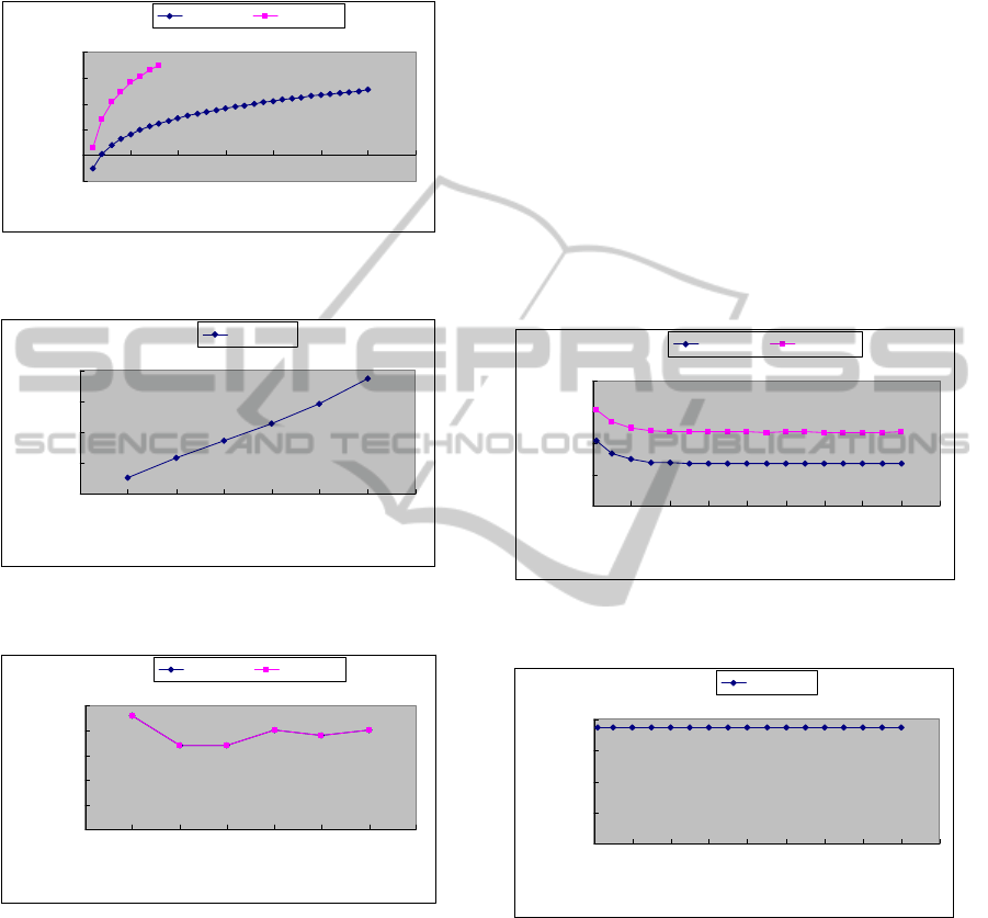
frequent patterns of UF-Evolve and FP-growth are
shown in Figure 18. The two algorithms mined the
same numbers and the same sets of frequent
patterns.
-1
0
1
2
3
4
00.511.522.533.5
Number of records (K)
Runtime (seconds)
(log scale)
UF-Evolve FP-growth
Figure 16: Runtime with number of records for UF-Evolve
and FP-growth.
0
500
1000
1500
2000
00.511.522.533.5
Number of records (K)
Number of shuffles
UF-Evolve
Figure 17: Number of shuffles with number of records for
UF-Evolve.
0
5
10
15
20
25
00.511.522.533.5
Number of records (K)
Number of mined frequent
patterns
UF-Evolve FP-growth
Figure 18: Number of mined frequent patterns with
number of records for UF-Evolve and FP-growth.
In the second experiment, we measured the
runtime, number of shuffles and number of mined
frequent patterns with different minimum support
thresholds for UF-Evolve and FP-growth. The
minimum support threshold varies from 0.1% to 8%,
the number of records is 3K, and the maximum
merging threshold is 0.3. The runtime of UF-Evolve
and FP-growth are shown in Figure 19. UF-Evolve
is faster and more scalable than FP-growth. When
the minimum support threshold increases, the
runtime of both UF-Evolve and FP-growth
decreases. Since when the minimum support
threshold is high, UF-Evolve processes fewer and
smaller conditional mUF-trees. The number of
shuffles of UF-Evolve is shown in Figure 20. When
the minimum support threshold increases, the
number of shuffles of UF-Evolve remains the same.
This is because UF-Evolve always shuffles the same
mUF-tree. The numbers of mined frequent patterns
of UF-Evolve and FP-growth are shown in Figure
21. The two algorithms mined the same numbers and
the same sets of frequent patterns. When the
minimum support threshold increases, the numbers
of mined frequent patterns of both UF-Evolve and
FP-growth decrease. This is because when the
minimum support threshold is high, the frequent
patterns are short and the set of such patterns is not
large.
0
2
4
6
8
0123456789
Minimum support threshold (%)
Runtime (seconds)
(log scale)
UF-Evolve FP-growth
Figure 19: Runtime with minimum support threshold for
UF-Evolve and FP-growth.
0
500
1000
1500
2000
0123456789
Minimum support threshold (%)
Number of shuffles
UF-Evolve
Figure 20: Number of shuffles with minimum support
threshold for UF-Evolve.
In the third experiment, we measured the number
of mined frequent patterns in each iteration for UF-
Evolve. The number of records is 3K, the minimum
support threshold is 0.1%, and the maximum
merging threshold is 0.3. As shown in Figure 22,
UF-Evolve discovers new frequent patterns from
iterative versions of mUF-tree, and the number of
mined frequent patterns keeps increasing until
stabilized.
For
the above experiments, UF-Evolve and FP-
UF-EVOLVE - UNCERTAIN FREQUENT PATTERN MINING
83

0
1
2
3
4
5
0123456789
Minimum support threshold (%)
Number of mined frequent
patterns (log scale)
UF-Evolve FP-growth
Figure 21: Number of mined frequent patterns with
minimum support threshold for UF-Evolve and FP-
growth.
0
5000
10000
15000
0 500 1000 1500 2000
Iteration
Number of mined frequent
patterns
UF-Evolve
Figure 22: Number of mined frequent patterns in each
iteration for UF-Evolve.
growth mined the same numbers and the same sets
of frequent patterns. Some of the discovered
frequent patterns are shown in Table 5. Here, the
supports for frequent patterns are shown as (support
count)/(number of records in UDB) in percentage.
Table 5: Discovered frequent patterns.
Frequent patterns
mined in 1
st
iteration
New frequent
patterns mined in
2
nd
iteration
New frequent
patterns mined in
3
rd
iteration
(59757:[0.3-0.3])
:4%
(45370:[0.7-0.7])
:5%
…
(29340:[0.1-0.3])
:3%
(59757:[0.3-0.4])
(22360:[0.3-0.3])
(18474:[0.5-0.7])
(29340:[0.1-0.3])
:3%
…
(45973:[0.2-0.3])
:4%
(38212:[0.8-0.8])
(8885:[0.2-0.5])
(45973:[0.2-0.3])
:4%
…
7 CONCLUSIONS
We have proposed the mUF-tree structure, which is
a novel uncertain-frequent-pattern discover
structure, and the UF-Evolve algorithm, which
utilizes the shuffling and merging techniques on the
mUF-tree for repeatedly discovering new uncertain
frequent patterns. Also, we proposed a variant of the
UF-Shuffle algorithms. Our preliminary
performance study shows that the UF-Evolve
algorithm is efficient and scalable for mining
additional uncertain frequent patterns with different
sizes of uncertain databases.
REFERENCES
Adnan, M., Alhajj, R., Barker, K., 2006. Constructing
Complete FP-Tree for Incremental Mining of
Frequent Patterns in Dynamic Databases. M. Ali and
R. Dapoigny (Eds.): IEA/AIE 2006, LNAI 4031, pp.
363 – 372, 2006.
Antova, L., Jansen, T., Koch, C., Olteanu, D., 2007. Fast
and Simple Relational Processing of Uncertain Data.
http://www.cs.cornell.edu/~koch/www.infosys.uni-
sb.de/publications/INFOSYS-TR-2007-2.pdf.
Borgelt, C., 2005. An Implementation of the FP-growth
Algorithm. OSDM’05, August 21, 2005, Chicago,
Illinois, USA.
Chau, M., Cheng, R., Kao, B., 2005. Uncertain Data
Mining: A New Research Direction. In Proceedings of
the Workshop on the Sciences of the Artificial,
Hualien, Taiwan, December 7-8, 2005.
Cheung, W., Zaiane, O. R., 2003. Incremental Mining of
Frequent Patterns Without Candidate Generation or
Support Constraint. Proceedings of the Seventh
International Database Engineering and Applications
Symposium (IDEAS’03).
Chui, C. K., Kao, B., Hung, E., 2007. Mining Frequent
Itemsets from Uncertain Data. Z.-H. Zhou, H. Li, and
Q. Yang (Eds.): PAKDD 2007, LNAI 4426, pp. 47–
58, 2007.
Ezeife, C. I., Su, Y., 2002. Mining Incremental
Association Rules with Generalized FP-Tree. R.
Cohen and B. Spencer (Eds.): AI 2002, LNAI 2338,
pp. 147–160, 2002.
Han, J., Pei, J., Yin, Y., Mao, R., 2004. Mining Frequent
Patterns without Candidate Generation: A Frequent-
Pattern Tree Approach. Data Mining and Knowledge
Discovery, 8, 53–87, 2004.
Hong, T. P., Lin, C. W., Wu, Y. L., 2008. Incrementally
fast updated frequent pattern trees. Expert Systems
with Applications 34 (2008) 2424–2435.
Leung, C. K. S., Carmichael, C., Hao, B., 2007. Efficient
Mining of Frequent Patterns from Uncertain Data.
ICDM-DUNE 2007.
Leung, C. K. S., Mateo, M. A. F., Brajczuk, D. A., 2008.
A Tree-Based Approach for Frequent Pattern Mining
from Uncertain Data. T. Washio et al. (Eds.): PAKDD
2008, LNAI 5012, pp. 653–661, 2008.
Li, H. F., Lee, S. Y., Shan, M. K., 2004. An Efficient
Algorithm for Mining Frequent Itemsets over the
Entire History of Data Streams. http://
citeseerx.ist.psu.edu/viewdoc/summary?doi=10.1.1.81.
9955.
IBM Quest Market-Basket Synthetic Data Generator.
http://www.cs.loyola.edu/~cgiannel/assoc_gen.html.
ICEIS 2011 - 13th International Conference on Enterprise Information Systems
84