
LOCALIZATION METHOD FOR LOW POWER
CONSUMPTION SYSTEMS
D. F. Larios, J. Barbancho, F. J. Molina and C. Le´on
Department of Electronic Technology, Escuela Polit´ecnica Superior, University of Seville, Seville, Spain
Keywords:
Localization, WSN, Fuzzy system, RSSI, Centroid, CL.
Abstract:
Locating nodes is a fundamental problem in wireless networks with hundreds of devices deployed in a wide
area. This is especially relevant for mobile nodes. Wireless sensor nodes are usually powered by small
batteries, solar panels or piezoelectric generators, so that, and consequently, power consumption is the main
constraint to deal with. But classic localization techniques do not consider the problem of energy consumption
as a key point. This paper presents a novel low power and range-free localization technique based on
distributed fuzzy logic and cooperative processing among a set of fixed nodes and its neighbours. This feature
permits better accuracy with less power consumption than most relevant localization techniques
1 INTRODUCTION
A wireless sensor network (WSN) consists of lots
of small devices deployed in a physical environment
for its study. Each node has special capabilities,
such as wireless communications with its neighbours,
sensing, data storage and processing.
WSNs have been widely used in many areas
(Akyildiz et al., 2002), such as environmental
monitoring (Yick et al., 2008), control (Riquelme
et al., 2009), healthcare and medical research (Chung
et al., 2008), national defense and military affairs (He
et al., 2004) (Boukerche et al., 2008), etc.
For most of these applications, it is usually
necessary to implement methods to estimate these
positions. In many cases, this information gathered
from the nodes is irrelevant without the knowledge of
the associated position, for example in WSN applied
to study wildfires (Antoine-Santoni et al., 2009). In
other applications, the node position is in fact the
required information (e.g vehicle tracking (Tubaishat
et al., 2009)).
Most important constraints for the design and
management of WSNs are data storage capability and
processing, weight (especially for mobile devices),
power consumption, cost, and radio coverage.
This paper presents LIS (Localization based on
Intelligent System), a novel localization algorithm
based on fuzzy logic processing. LIS is focused on
the reduction of energy consumption.
The paper is organized as follows: section 2 sums
up the state of the art about localization. Section 3
describes LIS. Section 4 shows the benefits of LIS
in power consumption. Simulations and the LIS
performance are summed up in section 5. Finally, in
section 6, we present concluding remarks and future
work.
2 LOCALIZATION TECHNIQUES
In localization applications, there are two types of
nodes:
• Anchor Nodes. Situated on fixed and known
positions.
• Non-anchor Nodes (Tags). Nodes with unknown
position. These nodes are usually called tags.
Localization algorithms presented in the literature
can be classified into two categories, as given below:
• Range-based. These techniques estimate,
point-to-point, the distance between each pair
of nodes. With this information and using
techniques, such as triangulation, the absolute
position of the non-anchor nodes can be
estimated. Generally, range-based techniques
require additional hardware. The most common
ones are Received Signal Strength Indication
(RSSI) (Awad et al., 2007), Time Of Arrival
(TOA) (Wu and Zhang, 2007) and Angle Of
Arrival (AOA) (Rong and Sichitiu, 2006).
22
F. Larios D., Barbancho J., J. Molina F. and León C..
LOCALIZATION METHOD FOR LOW POWER CONSUMPTION SYSTEMS.
DOI: 10.5220/0003518000220031
In Proceedings of the International Conference on Data Communication Networking and Optical Communication System (DCNET-2011), pages 22-31
ISBN: 978-989-8425-69-0
Copyright
c
2011 SCITEPRESS (Science and Technology Publications, Lda.)

• Range-free. The position of the non-anchor
nodes is obtained from the beacons sent by the
anchor nodes. Beacons contain information about
area coverage membership or number of hops
between devices. The most common range-free
techniques are Centroid (CL) (Bulusu et al., 2000)
and DV-Hop (Gao and Lei, 2010).
In general, the range-based ones offer good
accuracy, but additional hardware is often needed.
Therefore, the weight, the cost and the power
consumption of the node devices increase and
make these techniques unsuitable for the proposed
application. RSSI range-based techniques are an
exception to this because most of the current
transceivers provide this measurement by default.
However, RSSI techniques are very sensitive to noise
and interferences. Figure 1 shows experiments
to evaluate the relationship between RSSI and the
distance in different situations: free-space without
obstacles and long urban area with obstacles. The
results are expressed in absolute value.
0
10
20
30
40
50
60
70
80
90
100
5 10 15 20 25 30 35
RSSI
Distance (meters)
RSSI vs. Distance
With Obstacles
Free Space
Figure 1: RSSI vs. distance.
The results with obstacles do not match with any
valid mathematical model that could directly permit
to obtain the distance, using only the RSSI. Obtaining
models with the relationship between RSSI and
distance is currently an important area of research.
In any case, it is possible to obtain this model with
a much studied environment. However, the main
problem is to obtain the inverse of this relationship.
In fact different distances produced the same RSSI
value. Thus, even having a correct model of the
environment and ideal situations, it is not possible to
obtain the distance using only the RSSI information.
Instead of using a mathematical model, LIS
proposes a fuzzy-logic-based system to derive the
distance from RSSI level. This is more robust in noisy
and complex scenarios. The use of computational
intelligence in localization is not a novel idea, as
could be seen in previous works, such as (Rajaee
et al., 2008) that uses probabilistic neuronal networks,
(Xiufang et al., 2008) that applies a fuzzy system and
(Chiang and Wang, 2009) that uses fuzzy neurons.
In general, all these are distributed algorithms that
execute almost an important part of the localization
algorithm over the non-anchor nodes. However, none
of them consider the problem of power consumption
in the non-anchor nodes. Moreover, the algorithms
with Computational Intelligence generally track down
the current positions based on the estimated position
changes, needing an initialization of the non-anchor
nodes. These systems fail if the tags (the animal) go
out of the coverageof the WSN, and return into it after
a while.
3 LIS ALGORITHM
Despite the fact that the range-free and range-based
techniques have been extensively studied, nowadays
there are some aspects that continue to be a challenge:
• The use of additional hardware or lots of beacons
to increase power consumption.
• Fully centralized processing (i.e. on Base
Stations) requires a large amount of messages.
Conversely, processing in the tags’ nodes reduces
the battery of these devices significantly.
• Scalability. Manylocalization algorithms are hard
to extend to the big sensor networks.
LIS has been especially designed to phase out
all of the above mentioned problems. As a result,
the proposed algorithm is scalable and the power
consumption and network autonomy are optimized.
As usual in a tracking system, the non-anchor nodes
in LIS do not need to know their location, In this case,
only the Base Station wants to know it. LIS combines:
(1) a fuzzy system to estimate (actually to qualify) the
distance between transmitter and receiver from RSSI
measures, (2) a ubiquitous algorithm executed in
receiver anchor nodes to determine relative positions
to them, and (3) a cooperative algorithm to derive the
most likely location running at the Base Station.
LIS consists of four stages:
S1. Anchor nodes wait for non-anchor node beacons.
S2. The tag node broadcasts a beacon.
S3. Receiver anchor nodes measure RSSI, and
execute both, the fuzzification algorithm and
the ubiquitous processing for relative and partial
positioning.
S4. Anchor nodes send partial solutions to the Base
Station, where the location is finally determined.
LOCALIZATION METHOD FOR LOW POWER CONSUMPTION SYSTEMS
23
1 (B.S.)
2
3
4
5
6
7
8
(X?,Y?)
Anchor nodes
Non-anchor node
Communication link
Limit of radio coverage
Message transmission
(a)
1 (B.S.)
2
3
4
5
6
7
8
(b)
1 (B.S.)
2
3
4
5
6
7
8
(Xr7,Yr7)
(Xr4,Yr4)
(Xr5,Yr5)
(c)
1 (B.S.)
2
3
4
5
6
7
8
(Xr4,Yr4)
(Xr5,Yr5)
(Xr7,Yr7)
(X Y )
(X
Y ) Xr r
(d)
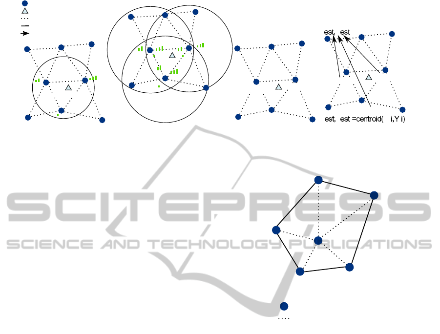
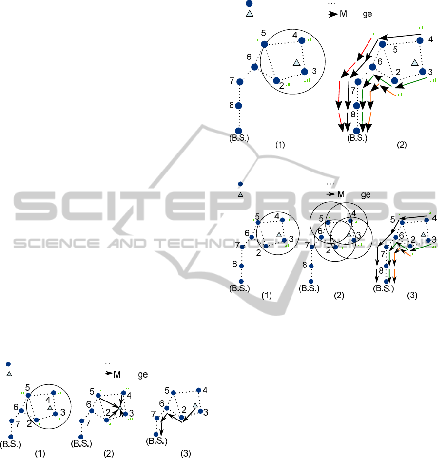
Figure 2: Steps of LIS algorithm.
Figure 2 illustrates these stages. When a
non-anchor node broadcasts a beacon or any other
sort of message, the localization process starts (figure
2.a). Just at that moment the receiver anchor nodes
participate in the process. The rest of the nodes can
switch off the radio transceiver or hold in it a low
power state.
3.1 Ubiquitous Processing
LIS uses the measured RSSI of a node and its
neighbors to determine the area where the non-anchor
node could be located. This algorithm is based on a
fuzzy system distributed on every anchor node of the
network.
According to the algorithm stages, once an anchor
node receives a beacon, it estimates the position of
the non-anchor nodes. The localization algorithm
has been designed to distribute the computation
consumption over the network. The area where
the non-anchor node could be localized with a
certain probability is called the Representative Area.
A “sector” is the minimum area formed by three
anchor-node neighbors. A Representative Area can be
made up of one or more sectors. Anchor nodes must
execute the distributed fuzzification algorithm for
every surrounding sector. Figure 3 shows an example
with five sectors, in which, the fuzzy algorithm is
executed five times.
Every anchor node that receives a beacon
measures and broadcasts the RSSI level to its anchor
neighbors (figure 2.b). In this way, the closest anchor
nodes elaborate a table with the RSSI measured by
themselves and their anchor neighbors.
The RSSI table is processed by the fuzzy system
to evaluate the Representative Area, irrespective of
the number of sectors. This area can be formed by
the union of one or more sectors (figure 2.c). A
sector is considered as a part of the Representative
Area if its membership degree is higher than the
Anchor nodes
Communication link
Neighbour 1
Sector
1
Sector
2
Sector
3
Sector
4
Neighbour 2
Neighbour 3
Neighbour 4
Sector
5
Neighbour 1
Figure 3: Example of node with 5 neighbours.
threshold. This value is adjusted experimentally.
The current simulations show that a threshold of 0.1
manages a good trade-off between the noise immunity
and localization performance. The results of the
Representative Areas are sent from the anchor nodes
to the Base Station to compute the final solution
(figure 2.d).
A Representative Area is empty if it does not
contain significant sector, i.e. if the membership
degree for all of them is lower than the threshold.
In this case, to save energy, the result is discarded
and the algorithm will finish until the next beacon
arrives (figure 4). This is especially important in huge
networks, where the energy needed for multi-hop
transmissions is high and is a disadvantage of the
centralized localization algorithm. This issue is
discussed in detail in section 4
3.1.1 The Fuzzy System Inputs
RSSI tables represent the signal level received in
either the local or the neighbor anchor nodes. Three
fuzzy sets qualify the RSSI as High, Medium and Low
DCNET 2011 - International Conference on Data Communication Networking
24

Anchor nodes
Non-anchor node
Communication link Limit of radio coverage
7
Message transmission
(B.S.)
n hops
Centraliced Algorithm
7
(B.S.)
n hops
Distributed Algorithm
In extended networks, redirect messages would waste a lot of energy
Some nodes sends
ierevelant information
to the Base Station
A node decides with our neighbour if it have relevant information
Nodes with no relevant
information do not send
messages to base station
Figure 4: Distributed algorithm would save Power Energy on extended networks.
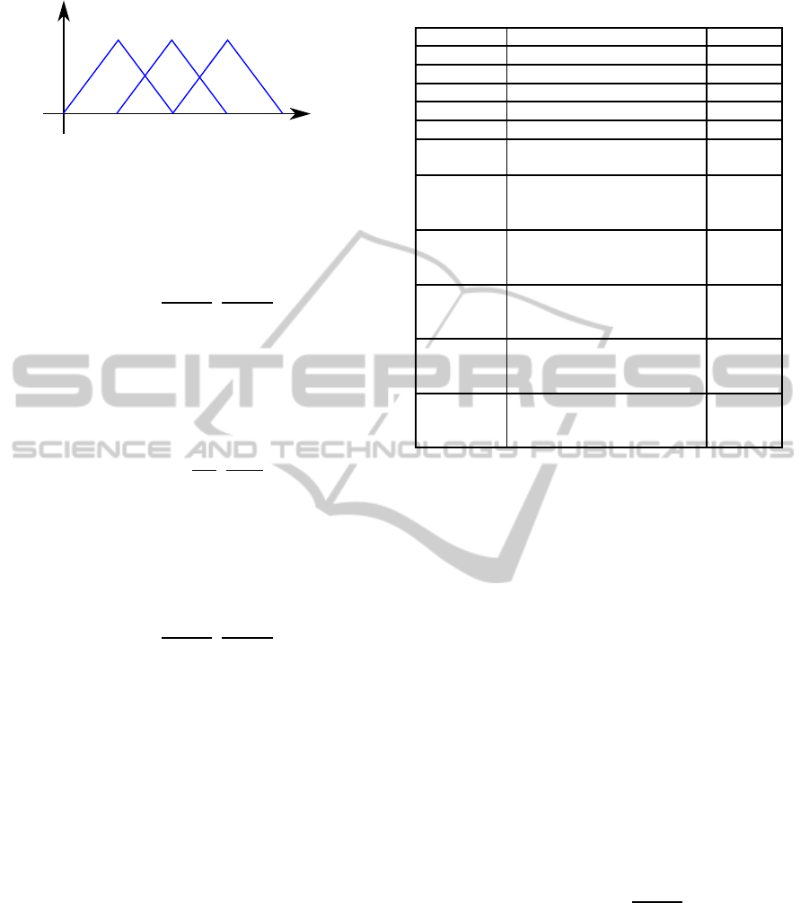
for each input (figure 5).
HIGH MEDIUM LOW
RSSI
med
RSSI
sens
RSSI
TX power
Figure 5: Sets of the fuzzy inputs.
The LOW RSSI fuzzy set is represented by a
trapezoid. The maximum membership degree (value
1) is assigned if the power falls down the sensibility
threshold of the emitter node (RSSI
sens
). As the power
increases, the membership degree decreases linearly
until it reaches zero. Following equation defines this
fuzzy set:
µ(x) = max
min
1,
a− x
a− b
,0
(1)
Where a = RSSI
med
and b = RSSI
sens
.
The medium RSSI fuzzy set is represented by
a triangle where the maximum membership degree
corresponds to the medium RSSI value (RSSI
med
).
The zero membership is reached for the power RSSI
values lower than the sensibility threshold or close
to the maximum transmission (RSSI
TXpower
). In
the current study, the medium RSSI value must be
computed for every sector using the Friis model
equation and assuming the emitter tag is located at the
centre. This computation only needs to be executed
once because the anchor nodes are located at fixed
positions.
P
RX
P
TX
= G
TX
· G
RX
·
λ
4πR
2
(2)
Where G
TX
and G
RX
are the gain of TX and RX
antennas, R is the distance between transmitter and
receiver and λ the wavelength.
The use of Friis is a trade-off between the
accuracy and the information required. More realistic
models require having more initial information of the
environment, a priori unknown, such as the position
of the obstacles. The Friis approximation simplifies
the problems of the saw-tooth of the disturbances
with a smooth function. According to a real scenario,
this assumption could not be a good approximation
to the reality. However, the errors assumed with
this approximation are compensated with the noise
immunity of LIS, which assumes the disturbances as
noise.
Next expression defines the fuzzy set for
MEDIUM RSSI:
µ(x) = max
min
x− a
b− a
,
c− x
c− b
,0
(3)
Where a = RSSI
sens
, b = RSSI
med
and c =
RSSI
TX power
.
Fuzzy set for HIGH RSSI values is a trapezoid
with a lineal increasing from 0 to 1 for the RSSI power
values ranging between RSSI
med
and RSSI
TX power
.
This fuzzy set is defined by the next expression:
µ(x) = max
min
x− a
b− a
,1
,0
(4)
Where a = RSSI
med
, b = RSSI
TXpower
.
3.1.2 The Fuzzy System Outputs
The Fuzzy System offers an output for each and every
sector. The output associated to a sector is a [0, 1]
ranged value that represents the confidence degree
that the tag is actually located in that sector.
LOCALIZATION METHOD FOR LOW POWER CONSUMPTION SYSTEMS
25
LOW MEDIUM HIGH
0 0.5 1
Figure 6: Sets of the fuzzy output.
As figure 6 shows, the LOW output fuzzy set is a
triangle with the central point at zero and the corners
at -0.5 and 0.5. Next expression defines this fuzzy set:
µ(x) = max
min
x+ 0.5
0.5
,
0.5− x
0.5
,0
(5)
The MEDIUM output is represented by a triangle
with the central point at 0.5 and corners at 0 and 1.
Mathematically it can be expressed by the following
equation:
µ(x) = max
min
x
0.5
,
1− x
0.5
,0
(6)
The HIGH output qualifier is also defined by a
triangle with the central point at 1 and the corners
at 0.5 and 1.5. This fuzzy set is defined by the next
expression:
µ(x) = max
min
x− 0.5
0.5
,
1.5− x
0.5
,0
(7)
3.1.3 Inference Engine
The inference engine is the Mandani’srules based one
with a centroid defuzzification method and a singleton
input fuzzificator. The fuzzy engine evaluates the
antecedent of every rule by the intersection of the
fuzzy inputs, using the minimum function for the
AND operator (Eq. 8), and the maximum function
for the OR operator (Eq. 9). The implication between
the inputs and outputs applies the minimum function.
AND(a,b) = min(µ(a), µ(b)) (8)
OR(a, b) = max(µ(a), µ(b)) (9)
As mentioned, the rules must be evaluated for
every single sector to estimate the confidence degree,
taking into account the fuzzy qualifications of RSSI
values of either the current sector nodes or the
surrounding ones. The rules summed up in Table 1
have been derived from multiple simulations in order
to obtain the best trade-off between precision and
noise immunity.
Table 1: Rules of the inference engine.
RSSI node RSSI Neighbours Output
High All medium High
Low All low Low
Medium All medium High
Medium All low Low
High All high Medium
Medium
Medium in current sector
High
Low in the rest
Medium
High in any sector except
the current one
Low
Low in the rest
High
High in a neighbour of the
current sector
Medium
Low in the rest
High
High in a neighbour, except
on the current sector
Low
Low in the rest
Medium
Medium in a neighbour of
the current sector.
Medium
Low in the rest
Medium
Medium in a neighbour,
except on the current sector
Low
Low in the rest
3.2 Cooperative Processing
The Base Station collects the partial solutions from
the anchor nodes, and processes them cyclically as
follows:
C1. The Base Station waits for receiving the first
partial solution.
C2. On arrival, the partial solution is saved and a timer
starts running.
C3. While the timer is running, the next partial
solutions are saved in a table as they were
received.
C4. When the timer expires, the system will compute
the final position as the centroid of all these
partial solutions (triangle sectors). The centroid
computation of a finite set of points
~
P
1
,
~
P
2
,· · ·
~
P
N
can be simplified as:
Position =
∑
N
i=1
~
P
i
N
(10)
The previous algorithm can be easily extended
to locating multiple tags, by simply associating a
tag identifier to the transmitted beacons. The final
estimated position is time stamped and saved in the
Base Station to make it accessible throughout the
Internet.
DCNET 2011 - International Conference on Data Communication Networking
26
4 POWER CONSUMPTION OF
LIS
Generally, power consumption is a strong constraint
in a WSN application. This is especially true in
mobile target tracking (e.g. wild animals in natural
environments). Power constraints are higher for
non-anchor or mobile nodes. Anchor nodes can
recharge their batteries, using systems as such as
solar panels. But for non-anchor nodes, mobility
and additional constraints like size and weight do
not allow use of high capacity batteries or any other
alternative power source.
Most node power consumption is caused by
radio transmissions. As an example, the Telosb
platform consumes 41 mW in active mode. The
microcontroller consumes only 5 mW and the
remainder power consumption is caused by the radio
transceiver that requires 38 mW in the receiver mode
and 35 mW in transmission (Polastre et al., 2005).
It is important to point out that the power
consumption is very high either in transmission or in
the reception mode. Therefore, to reduce the power
consumption it is necessary to reduce the number of
exchange messages, and also stop all the node activity
enabling low power modes and switch on the radio
transceiver. Therefore, a suitable activity manager
with hibernation periods is needed. This problem is
analysed later.
Figure 7 represents a localization algorithm
computed in the non-anchor node.
Anchor nodes
Non-anchor node
Communication link
essa transmission
Figure 7: Localization algorithm using the non-anchor node
for estimate its positions.
As it can be observed, after the tag node
broadcasts a beacon 7.1), it should wait for the
response of all the anchor nodes placed in the radio
range (7.2). This phase takes a long time because
of the number of surrounding nodes and also the
collisions. After that, the tag node executes the
localization algorithm and delivers the result to the
Base Station (7.3). During all of this, the radio
transceiver must be in the active state. It wastes a lot
of energy and the autonomy is considerably reduced
Anchor nodes
Non-anchor node
Communication link
essa transmission
Figure 8: Example of centralized algorithm.
Anchor nodes
Non-anchor node
Communication link
essa transmission
Figure 9: Example of distributed algorithm.
for the non-anchor node. It is in fact, the device with
higher energy constraints.
LIS takes this issue into account. Also, that anchor
nodes have more power supply resources than the
tags. The algorithm has been designed to be executed
mainly in the anchor nodes. Furthermore, the radio
transceiver of the tag is activated for a short time, just
enough to broadcast the beacon. In the remaining
period of time, the tag will be in a idle state and its
radio transceiver off.
But LIS also reduces the power consumption in
anchor nodes. It implements an ubiquitous and
distributed algorithm that spreads the localization
processing amongst the nodes surrounding the tag.
In a centralized-only algorithm, all the information
received by the anchor nodes must be delivered
to the Base Station (Figure 8). By contrast,
proposed algorithm saves power energy because only
significant information is delivered (Figure 9).
In the worst case, LIS delivers practically the same
number of messages than a centralized algorithm.
But for low dense deployments, for example when
medium number of nodes that a beacon receives is
lower than the medium number of hops necessary to
reach the Base Station, the savings is significant.
LOCALIZATION METHOD FOR LOW POWER CONSUMPTION SYSTEMS
27
0
5
10
0
5
10
0
10
20
30
40
2 Hops
Number of nodes with
useful information
Number of nodes
Total amount of transmissions
Centralized
Distributed
(a)
0
5
10
0
5
10
0
20
(b)
0
5
10
0
5
10
0
50
100
150
Centralized
Distributed
10 Hops
Number of nodes with
useful information
Number of nodes
Total amount of transmissions
(c)
Figure 10: Messages transmission versus the number of nodes: A) Two hops, B) 6 hops, C) 10 hops.
As a consequence, the energy saved with the
distributed algorithm varies with the density and
complexity of the networks. Figure 10 shows a
study about the number of delivered messages in
function of the number nodes with useful information.
From this, it can be derived that in case that
all the information obtained by the anchor nodes
were useful, both methods send practically the same
number of messages. But the more number of
nodes with useless information, the energy saving
performance of the distributed processing increases
drastically.
Additional savings can be managed by clustering
the networks, and using the cluster heads as the
Base Stations, i.e. receiving the processing partial
estimations from its cluster nodes. Figure 11 shows
this idea.
Anchor nodes
Non-anchor node
Messa
Figure 11: Example of the use of clusters.
For this case, the algorithms must be modified as
follows:
S1. Anchor nodes wait for non-anchor node beacons.
S2. The tag node broadcast a beacon.
S3. Receiver anchor nodes measure RSSI, and
execute both, fuzzification algorithm and
ubiquitous processing for relative and partial
positioning.
S4. Anchor nodes send partial solutions to the
clusterhead, where the location is finally
determined
S5. Clusterhead node executes the cooperative
positioning algorithms and delivers the final
position to the Base Station.
S6. Base Station executes the same cooperative
positioning algorithm than the clusterhead nodes,
but using the information delivered from these
clusterheads. In this way, if the tag positioning
comes from just one clusterhead, this position will
be considered as the final solution. But, if it
is received from more than one clusterhead, the
centroid estimation is applied to all of them.
Determining when the use of clustering saves
more energy is not trivial. It depends on the size
and complexity of the network. But in general, it
is reasonably to think that clustering techniques are
better for wide and complex networks.
Additionally, a distributed processing such as the
one proposed in this paper, increases Throughput and
reduces the response delay, because traffic bottleneck
and collisions close to the Base Station are avoided.
Distributed processing also spreads computational
load over the network. This is especially important
for wide networks or with multiple non-anchor nodes.
5 ACCURACY OF LIS
The accuracy of LIS versus the classic CL algorithm
(Bulusu et al., 2000) was compared using different
simulations. The election of centroid as the reference
algorithm to compare with is based on the fact that
many authors use it in their research studies. Thus, it
is possible to obtain a conclusion on the accuracy of
LIS not only with the centroid, but also with all the
DCNET 2011 - International Conference on Data Communication Networking
28
other localization techniques that are compared with
it in the literature.
The tested network was made up of 25 anchor
devices with a radio range of 200 meters in a
non-anchor node and with separated anchor nodes
also with a radio range of about 200 meters. The
anisotropic radiation pattern was assumed. The
simulator has been developed in C++. It allows
the selection of the radio range, radiation pattern,
Gaussian noise, sensibility, network deployment and
anchor location. All the parameters, in the tests
have been selected to model the Telosb devices and
using a Friis propagation model. The results of the
simulations are presented in the next subsection.
The use of a simulator for obtaining the accuracy
of a localization algorithm is a common tool. It
is difficult to compare the localization algorithms
in real scenarios, because of the changes of the
environment. Thus, these experiments are generally
not replicable, even by the author (different days
would offer different results). Obtaining unified
comparison criteria for the localization algorithm
and the necessary parameters to consider in the
real experiments is currently an important area of
research, which is far from over. However, simulation
results are easily reproducible and permit the
comparison of the localization algorithms amongst
themselves.
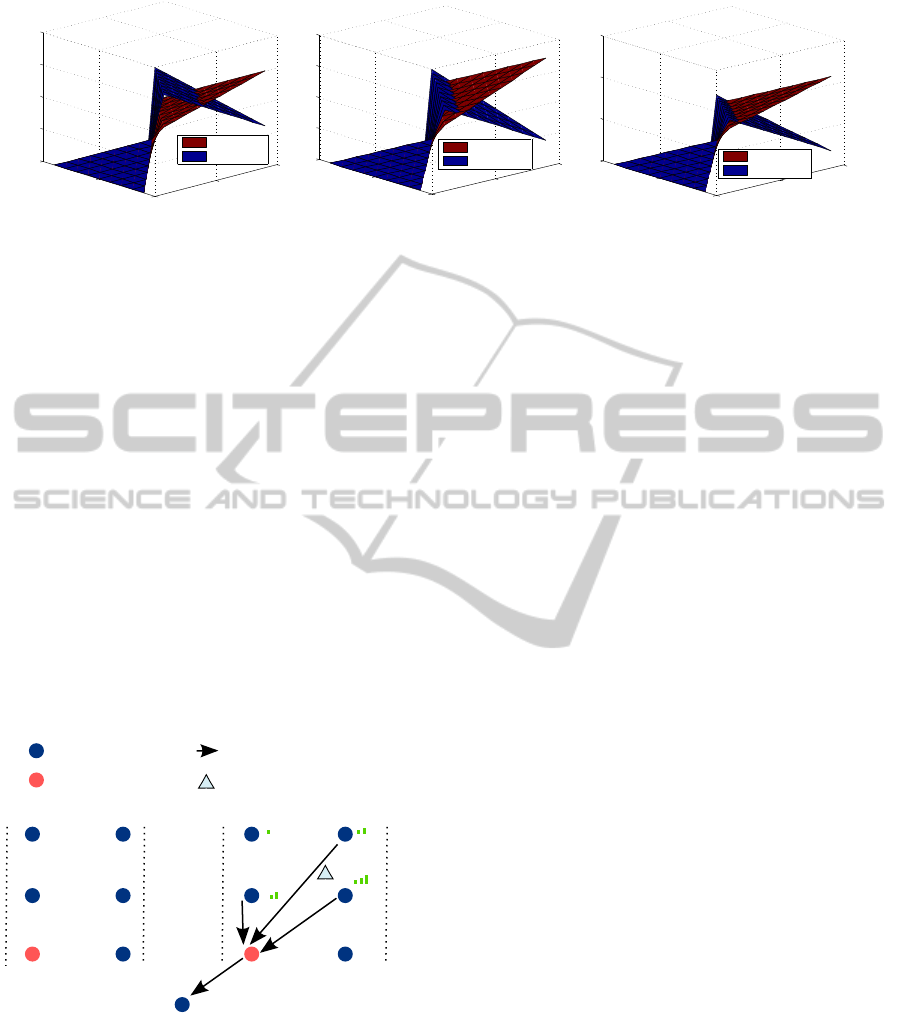
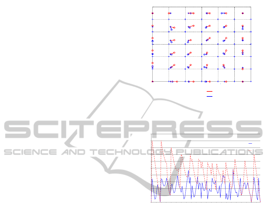
5.0.1 Error vs. Position
The following experiments include a moving tag into
the network. The noise has been neglected and
the error is expressed in meters. As figures 12
and 13 show, the maximum end medium errors of
LIS algorithm are considerably smaller than the ones
estimated with the (CL) Centroid classic algorithm.
Figure 12 is a graphical representations of the
errors, which represents the real position and the
estimated position of the algorithms in a few analyses.
The results are normalized with the radio coverage
of the non-anchor nodes that are 200 meters in these
tests.
Figure 13 represents the position error, measured
as the absolute value of the Euclidean distance
between the real and the estimated position. The
results are normalized with the non-anchor node radio
range. They are obtained by moving the non-anchor
node into the quadrant made up by the anchor nodes
7, 8, 9 and 12, in a step of 2 meters. The X axis
represents the relative position of the tag into the
quadrant, assuming that node 8 is the coordinates
origin. These values are normalized with the distance
between then nodes (200 meters). The last relative
point simulated is [0.5 0.5] because the other three
o
Estimated CL Possition
Estimated LIS Possition
Error of LIS
Error of CL
*
Position of non-anchor node
+
Position of anchor nodes
0
1
2
3
4
5
6
0 1 2 3 4 5 6
Figure 12: Position error of CL algorithm and LIS
algorithm.
LIS
CL
Error vs. Possition
Location error (% non-anchor node radio range)
50%
45%
40%
35%
30%
25%
20%
15%
10%
5%
0%
Non-anchor node possition (Relative to distance between anchor nodes)
0
0
Y
X
0.05
0
0.1
0
0.15
0
0.2
0
0.25
0
0.3
0
0.35
0
0.4
0
0.45
0
0.5
0
0.5
0.5
Figure 13: Localization error vs. the position of the
non-anchor node.
parts of the quadrant offer symmetrical results than
obtained result.
5.0.2 Error vs. Coverage
Figure 14 shows the influence of the radio range. As
the radio range increases, the number of non-anchor
nodes that receive a beacon also increases, and the
error decreases. In this scenario the noise has not been
considered. The radio range of the non-anchor node
simulated is in the [100 m - 350 m] range.
Results are the relative error to the distance
between the anchor nodes that are separated 200
meters. There are six different points, which
are simulated corresponding to the points 1 to 6
represented in the figure, separated by 50 meters.
These points are into the quadrant of the nodes 7,
8, 12 and 13 of the network. The rest of the points
can be obtained by dividing the quadrant in step of 50
meters, which offers identical results than those of the
LOCALIZATION METHOD FOR LOW POWER CONSUMPTION SYSTEMS
29

simulated. This is because of the symmetry.
Anchor nodes
Non-anchor node itions
7
8
1312
1 2 3
4 5
6
Coverage of non-anchor node (meters)
0%
10%
20%
30%
40%
100 140 180 220 260 300 340
4
Coverage of non-anchor node (meters)
0%
10%
20%
30%
40%
100 140
180 220 260 300 340
5
Coverage of non-anchor node (meters)
0%
10%
20%
30%
40%
100 140 180 220 260 300 340
6
Coverage of non-anchor node (meters)
Location error
0%
10%
20%
30%
40%
100 140 180 220 260 300 340
3
Coverage of non-anchor node (meters)
0%
10%
20%
30%
40%
100 140 180 220 260 300 340
1
Coverage of non-anchor node (meters)
0%
10%
20%
30%
40%
100 140 180 220 260 300 340
2
LIS
CL
LIS
CL
LIS
CL
LIS
CL
LIS
CL
LIS
CL
Location error
Location error
Location error
Location error
Location error
Figure 14: Localization error vs. the coverage radio area of
non-anchor node.
In all of the cases, LIS gets smaller or equal
errors than the centroid algorithm. Similar results
are obtained by fixing the coverage area of the
non-anchor nodes and reducing the distance between
the anchor devices from the simulated 200 meters.
These results are similar to the evaluation of the error
versus the node density, which was proposed by the
other authors.
As it can be seen in points where there is
symmetry between the position of the tags and the
anchor nodes (points 1, 3 and 6), the error is always
0 for all the simulated coverage. This is a typical
behavior of the centroid, which has low errors in these
symmetrical points, but has very bad behavior outside
these points. LIS presents a good behavior in all of the
simulated points.
With the two algorithms, better accuracy is
obtained by increasing the number of anchor nodes
that receives the beacon, but with the proposed
method, the system tends to lower the errors earlier.
6 CONCLUSIONS AND FUTURE
WORK
LIS is a new fuzzy algorithm for localization designed
to reduce power consumption, especially but not
limited to, the tag nodes where the power constraints
are higher. LIS filters the useless information
after being processed in the anchor nodes. It also
implements a hibernation mechanism. All these
mechanisms increase the battery autonomy.
LIS has been tested by simulations. The obtained
results showed that the proposed method obtains less
localization errors than the CL algorithm without
higher computation requirements or an extensive use
of radio.
The localization system LIS is being applied to
locating and tracking of wild animals in natural parks.
ACKNOWLEDGEMENTS
This research has been supported by the “Consejer´ıa
de Innovaci´on, Ciencia y Empresa”, “Junta de
Andaluc´ıa”, Spain, through the excellence project
ARTICA (reference number: P07-TIC-02476) and by
the “C´atedra de Telef´onica, Inteligencia en la Red”,
Seville, Spain, through the project ICARO.
The authors would like to thank the Biological
Station of the natural park of “Do˜nana” and the
researchers of its Biological Station Centre, for their
collaboration and support.
REFERENCES
Akyildiz, I. F., Su, W., Sankarasubramaniam, Y., and
Cayirci, E. (2002). Wireless sensor networks: A
survey. Computer Networks, 38(4):393–422.
Antoine-Santoni, T., Santucci, J. F., de Gentili, E., Silvani,
X., and Morandini, F. (2009). Performance of a
protected wireless sensor network in a fire. analysis
of fire spread and data transmission. Sensors,
9(8):5878–5893.
Awad, A., Frunzke, T., and Dressler, F. (2007). Adaptive
distance estimation and localization in wsn using
rssi measures. In 10th Euromicro Conference on
Digital System Design Architectures, Methods and
Tools, DSD 2007, pages 471–478. Sponsors: Drager;
Conference code: 72733; Cited By (since 1996): 11.
Boukerche, A., Oliveira, H. A. B. F., Nakamura, E. F.,
and Loureiro, A. A. F. (2008). Secure localization
algorithms for wireless sensor networks. IEEE
Communications Magazine, 46(4):96–101. Cited By
(since 1996): 11.
Bulusu, N., Heidemann, J., and Estrin, D. (2000). Gps-less
low-cost outdoor localization for very small devices.
IEEE Personal Communications, 7(5):28–34.
Chiang, S. Y. and Wang, J. L. (2009). Localization in
wireless sensor networks by fuzzy logic system. In
13th International Conference on Knowledge-Based
and Intelligent Information and Engineering Systems,
KES 2009, volume 5712 LNAI, pages 721–728.
DCNET 2011 - International Conference on Data Communication Networking
30

Chung, W. Y., Lee, Y. D., and Jung, S. J. (2008).
A wireless sensor network compatible wearable
u-healthcare monitoring system using integrated ecg,
accelerometer and spo2. In 30th Annual International
Conference of the IEEE Engineering in Medicine and
Biology Society, EMBS’08, pages 1529–1532.
Gao, G. Q. and Lei, L. (2010). An improved node
localization algorithm based on dv-hop in wsn. In
Northeastern University, volume 4, pages 321–324.
He, T., Krishnamurthy, S., Stankovic, J. A., Abdelzaher,
T., Luo, L., Stoleru, R., Yan, T., Gu, L., Hui, J.,
and Krogh, B. (2004). Energy-efficient surveillance
system using wireless sensor networks. MobiSys 2004
- Second International Conference on Mobile Systems,
Applications and Services, pages 270–283.
Polastre, J., Szewczyk, R., and Culler, D. (2005). Telos:
enabling ultra-low power wireless research. In
Information Processing in Sensor Networks, 2005.
IPSN 2005. Fourth International Symposium on,
pages 364 – 369.
Rajaee, S., Almodarresi, S. M. T., Sadeghi, M. H., and
Aghabozorgi, M. (2008). Energy efficient localization
in wireless ad-hoc sensor networks using probabilistic
neural network and independent component
analysis. In 2008 International Symposium on
Telecommunications, IST 2008, pages 365–370.
Riquelme, J. A. L., Soto, F., Suard´az, J., S´anchez,
P., Iborra, A., and Vera, J. A. (2009). Wireless
sensor networks for precision horticulture in southern
spain. Computers and Electronics in Agriculture,
68(1):25–35.
Rong, P. and Sichitiu, M. L. (2006). Angle of arrival
localization for wireless sensor networks. In Sensor
and Ad Hoc Communications and Networks, 2006.
SECON ’06. 2006 3rd Annual IEEE Communications
Society on, volume 1, pages 374–382.
Tubaishat, M., Peng, Z., Qi, Q., and Yi, S. (2009). Wireless
sensor networks in intelligent transportation systems.
Wireless Communications and Mobile Computing,
9(3):287–302.
Wu, S. H. and Zhang, N. T. (2007). Two-step toa estimation
method for uwb based wireless sensor networks. Ruan
Jian Xue Bao/Journal of Software, 18(5):1164–1172.
Xiufang, F., Zhanqiang, G., Mian, Y., and Shibo, X.
(2008). Fuzzy distance measuring based on rssi in
wireless sensor network. In Proceedings of 2008 3rd
International Conference on Intelligent System and
Knowledge Engineering, ISKE 2008, pages 395–400.
Yick, J., Mukherjee, B., and Ghosal, D. (2008).
Wireless sensor network survey. Computer Networks,
52(12):2292–2330.
LOCALIZATION METHOD FOR LOW POWER CONSUMPTION SYSTEMS
31
