
TARGET-AWARE ANOMALY DETECTION AND DIAGNOSIS
Alexander Borisov
1
, George Runger
2
and Eugene Tuv
1
1
Intel, Chandler, AZ, U.S.A.
2
Arizona State University, Tempe, AZ, U.S.A.
Keywords:
Outliers, Process control, Contribution plots, Partial least squares.
Abstract:
Anomaly detection in data streams requires a signal of an unusual event, and an actionable response requires
diagnostics. Furthermore, monitoring for process control is often concerned with one or more target (con-
trolled) attributes. Consequently, it is necessary to separate anomalies (and their contributing attributes) that
could influence the controlled target strongly, and this becomes more important with the increased number
of monitored attributes in modern processes. This task leads to a difficult problem not addressed directly by
the machine learning/process control community. We introduce the target-aware anomaly detection problem
and present a solution for process control in modern systems (with nonlinear dependencies, high dimensional
noisy data, missing data, and so on). The main objective is to identify and rank outliers and also diagnose
their contributing attributes with respect to the possible effect on the response. The method is different from
traditional linear and/or univariate approaches, as it can deal with local data structure in the neighborhood of
an outlier, and can handle complex interactions via the use of an appropriate learner. In addition, the method
can be computed quickly and does not require time consuming matrix operations. Comparisons are made to
traditional contribution plots computed from partial least squares.
1 INTRODUCTION
The importance of anomaly detection has grown from
manufacturing to include systems such as environ-
mental, security, health, supply chains, transportation,
etc. Data are characterized by a set of input attributes
(or variables), and one (or several) controlled (target)
attribute(s). A typical example of an input set con-
sists of measurements generated over different stages
of a production process from numerous sensors (from
hundreds to thousands). Along with the input mea-
surements target attributes may result from final prod-
uct tests or other system performance measures. The
usual goal of the process control is to keep the values
of the target attributes within a given range. Further-
more, if we observe or predict an excursion in a target,
it is important to determine what inputs contribute to
the excursion.
In applications (such as process control) where the
objective is to control a target attribute, and as the
number of input attributes increase, it becomes im-
portant to focus anomaly detection to the effect on the
target. Furthermore, although target-labeled training
data is used, we do not assume that the process data is
target-labeled when the outlier diagnostics are comp-
uted. For many common process control applications
the decision for action must be based on the input at-
tributes before the target is measured. Consequently,
we refer to our approach as target-aware, rather than
supervised.
This problem has not been addressed in the ma-
chine learning literature. Instead, commonly used
methods in advanced process control applications (for
both unsupervised and supervised anomaly detection)
rely on linear data models (i.e., principal component
analysis (PCA) and partial least squares (PLS) (Hastie
et al., 2001)) and multivariate normal distribution as-
sumptions in the input space. Such approaches (e.g.,
for example, (Ergon, 2004)) can be successful in find-
ing anomalies in low-dimensional, non-noisy numeric
data when the dependency between the inputs and
outputs are near-linear. PLS provides an approach for
target-labeled outlier detection and attempts to iden-
tify input attributes that most strongly contribute to
an outlier. However, the above strong assumptions
limit the applicability for data that can be very large
(millions of samples and/or several hundreds to thou-
sands of predictors), noisy, with heterogeneous type
(numerical and categorical). Other anomaly detection
approaches (e.g., see reviews by (Hodge and Austin,
14
Borisov A., Runger G. and Tuv E..
TARGET-AWARE ANOMALY DETECTION AND DIAGNOSIS.
DOI: 10.5220/0003530100140023
In Proceedings of the 8th International Conference on Informatics in Control, Automation and Robotics (ICINCO-2011), pages 14-23
ISBN: 978-989-8425-74-4
Copyright
c
2011 SCITEPRESS (Science and Technology Publications, Lda.)

2004)) can not be easily extended to supervised set-
tings.
Solutions to the problem above can be approached
in several ways. One is to build a model on previously
seen data that is capable of predicting failures or large
changes in a target from recently arrived new data.
We refer to this as predictive modeling. Such an ap-
proach based on different types of regression models
was used in an off-line setting (Angelov et al., 2006).
However, an important concern is that such models
may generalize poorly on new data when the distri-
bution of inputs changes. To address this concern
previous work considered adaptive models were up-
dated based on new test data that were determined to
be fault-free (Lughofer and Guardioler, 2008; Filev
and Tseng, 2006). An advantage of our approach is
that the model need not be updated and we integrate
unsupervised information.
An alternative is unsupervised anomaly detection
where the objective is to find points in input space that
are distant from the ”general” input distribution, thus
effectively detecting anomalies in new (or existing)
data (Chiang et al., 2001). However, such an anomaly
in the input attributes might (but does not always) lead
to a large change in the target value too. Still there
is not a direct link between the two, as the unsuper-
vised nature of anomaly detection does not take into
account the predictive model that is used.
We propose a novel target-aware anomaly detec-
tion approach that combines both predictivemodeling
and unsupervised outlier detection. We use a predic-
tive model learned from target-labeled training data
to assign ”outlier scores” to new data points. These
scores consider both the effect on the target as well as
the remoteness of point in the space of inputs. (Note
that this is different from predicting target probabili-
ties from the model directly, as those probability es-
timates also do not generalize outside of the current
input distribution.) Furthermore, we propose a mea-
sure that separates the most influential outliers, and
ranks them according to influence on the target, along
with a threshold used to filter the non-influential out-
liers and normal samples. As an important by-product
for signal diagnosis, we compute the contribution of
input attributes to the anomaly score. This task is re-
lated to fault isolation and several methods have been
used (Efendic et al., 2003; Runger et al., 1996). We
propose a ranking measure, along with a threshold, to
identify the input attributes that contribute to a partic-
ular point being an outlier. Our analysis statistically
quantifies risks and we use quite different models and
metrics than previous work.
Regarding terminology, we note that supervised
and unsupervised anomaly detection can refer to
whether samples are labeled as normal or anomalous
and not the target attribute labels (Chandola et al.,
2009). Consequently, we refer to our method as
target-aware anomaly detection. We performed ex-
periments with simulated data sets that closely mimic
the behavior of real systems and show that our method
outperforms classical PLS contribution plot analysis,
both in terms of detecting outliers, calculating rel-
evant contributions, and in terms of improving pre-
dictive accuracy on new data when potential outliers
are detected automatically even before the target is
known. The algorithm was successfully applied on
real data too. Here we focus on the case of a nu-
merical target (regression case) with numerical inputs
because it is more relevant for statistical process con-
trol. We provide a short description of traditional PLS
based anomaly detection approach in Section 2. Sec-
tion 3 presents our new method. Section 4 offers il-
lustrative examples and compares to the traditional
PLS contribution plots, and Section 5 provides con-
clusions.
2 TRADITIONAL LINEAR
METHODS FOR SUPERVISED
ANOMALY DETECTION
The supervised outlier detection and contribution
problem has been addressed in the statistical litera-
ture through linear models with PLS regression (Wold
et al., 2001). The PLS approach is the only method
that has been been applied for outlier/contribution
analysis in the supervised case. PLS iteratively
computes components (directions) with maximum
correlation to the target, performing Gram-Schmidt
orthogonalization of the input space and the tar-
get with respect to the new identified component.
The process continues until a predefined number of
components is generated. In this way it yields a
number of mutually orthogonal directions that have
maximum correlation to the target. Projections of
the input space along these directions yield load-
ings/projection/scores (similar to PCA). PLS results
in the regression coefficients for target y with respect
to these directions.
More formally, a PLS model has the form X =
TP
t
, y = TQ
t
, where P, Q are X and y loadings, re-
spectively, and t denotes matrix transpose. Here T is
the score matrix with columns corresponding to di-
rections. So in addition to finding a new basis in X
space it provides a regression model for y. Similar to
PCA, a PLS model is sensitive to the scaling of at-
tributes, and therefore requires an appropriate scale
TARGET-AWARE ANOMALY DETECTION AND DIAGNOSIS
15

to be selected. In most applications the attributes are
standardized (zero mean and unit standard deviation)
and for simplicity we make this assumption in this
paper. The PLS algorithm description can be found,
for example, in (Hastie et al., 2001). The number of
directions is usually selected using an explained vari-
ance threshold or cross-validation.
Two common statistics are used to monitor for
anomalies (similar to the PCA case). First is squared
prediction error (SPE). That is, the distance from an
inspected sample to the model plane defined by se-
lected latent variables. Second is the distance from
zero (the center of the scaled distribution) in score
space. To account for different score scales, and their
different influence on the target, scores are multiplied
by the corresponding y-loadings and divided by the
standard deviation. More insight on these two mea-
sures follows next.
Suppose we computed and selected K directions
{T
1
, T
2
, .. . , T
K
} from a PLS model given by X =
TP
t
, y = TQ
t
, where T = T(N ×K), P = P(N ×
K), Q = Q(1×K) matrices. Let the kth column of
TandQ be denoted as T
k
and Q
k
, respectively. Here
Q denotes the coefficient estimates from the linear re-
gression of y on T and the (scalar) Q
k
is a measure
of the weight of T
k
in the regression. A modified
Hotelling’s T
2
statistic (Hotelling, 1947) with respect
to selected components is computed as follows:
T
2
=
K
∑
k=1
T
k
·Q
k
λ
k
2
, (1)
where λ
k
is the standard deviation of the elements of
T
k
. Here T
2
is similar to the (Mahalanobis) distance
of data sample x
x
x
0
from the centroid
¯
x
x
x after a projec-
tion to the subspace defined by the first K latent vari-
ables. An anomaly is signaled if this distance is too
large. However, multiplication by the y-loadings Q
allows one to take into account the influence of com-
ponents on the target.
Because T
2
statistic is not sensitive to anomalies
that are far from the subspace of the latent variables,
a second statistic is used that is sensitive to the dis-
tance from this subspace. Suppose R = R(N ×K) is
the projection matrix from the original input space to
scores, i.e T = XR, P
t
R = I. The squared prediction
error (SPE) is
SPE
0
= (x
x
x
0
−
ˆ
x
x
x
0
)
t
(x
x
x
0
−
ˆ
x
x
x
0
) (2)
where
ˆ
x
x
x
0
= x
x
x
0
RP
t
is the projection of x
x
x
0
to the sub-
space spanned by the first K PLS components in the
input space.
We define the (supervised) PLS contribution score
of attribute j to data sample x
x
x
0
to T
2
, in a manner
similar to (Ergon, 2004) and (Miller et al., 1998),
but scores are multiplied with their corresponding y-
loadings. That is,
C
j
(T
2
, x
0
) = x
0j
·
v
u
u
t
K
∑
k=1
T
k
Q
k
·R
jk
λ
k
2
(3)
and this can be interpreted as the multiplication of the
scores (normalized and weighted by y-loadings) by
the term x
0j
R
jk
that gives influence of attribute j on
the score T
k
= XR
k
.
Similarly, the PLS contribution score of attribute
j for x
x
x
0
to SPE is calculated from the j-th term of (2)
in the same way as for PCA model. That is,
C
j
(SPE, x
0
) = (x
0j
− ˆx
0j
)
2
(4)
3 TARGET-AWARE ANOMALY
AND CONTRIBUTOR SCORING
ALGORITHM
As stated earlier, the notion of ”target-aware out-
lier/anomaly detection” is closely related to the effect
on a target. More precisely, call an outlier in X space
an influential outlier if it has a large influence on the
target. Call all other outliers (with minor or no influ-
ence on the target) non-influential outliers. For ex-
ample, an outlier in an irrelevant attribute will have
no influence. Our goal here is to detect influential
outliers and determine the attributes that contribute to
them. We assume training data with target-labels for
a predictive model, but to meet the conditions in pro-
cess control applications we assume that target values
are not available at the time anomaly detection is eval-
uated.
Due to the complexity and size of real data sets,
and to address nonlinear models, interactions, miss-
ing data, different units for attributes, and other prop-
erties of practical problems, we develop new scores
and diagnostics from tree based models. An ensem-
ble of gradient boosting trees models (GBT) (Fried-
man, 2001) is used to calculate a ”target-aware outlier
score”, that describes how well a new (or old) sample
fits into the input distribution partitioned by trees in
the model with adjustment for the target.
3.1 Decision Tree Formulas
We consider the practical case where both the input
attributes and the target are continuous. A decision
tree provides a supervised predictive model (Breiman
et al., 1984) that recursively partitions samples to
achieve smaller impurity of the target attribute. The
samples at a node are partitioned (split) into subsets at
ICINCO 2011 - 8th International Conference on Informatics in Control, Automation and Robotics
16

the two child nodes (because we only consider binary
trees). Each split is defined by a binary rule on one
of the input attributes X
j
. For a continuous attribute
partitions of the form X
j
< v or X
j
> v are considered.
The attribute for which the binary rule minimizes the
impurity of the target is called the primary (best) split-
ter. The impurity is measure defined by entropy or the
Gini index for categorical targets and for a numerical
target we use squared error loss
I(T) =
∑
i∈T
(y
i
− ¯y(T))
2
where ¯y is the mean of the target values at the node.
After a split the impurity of the two child nodes is
computed as
I(T
L
) + I(T
R
) =
∑
i∈T
L
(y
i
− ¯y(T
L
))
2
+
∑
i∈T
R
(y
i
− ¯y(T
R
))
2
where ¯y(T
L
) and ¯y(T
R
) are the target means in the left
and right child nodes, respectively. The change in
impurity from the parent to the child nodes obtained
from the primary splitter is denoted as
W(T) = I(T) −I(T
L
) −I(T
R
) (5)
and referred to as the split weight. Larger values indi-
cate a more important split at node T.
The process continues until a stopping rule is true.
A single tree algorithm might further prune (remove)
nodes, but typically ensemble models do not. Given
a sample x
0
the attribute values in x
0
determine a
path through the nodes until a terminal (leaf) node is
reached. The majority class of the target at the leaf is
often used to predict a categorical target and the mean
of the target values at a leaf is often used to predict a
continuous target. A GBT model is a (serial) ensem-
ble of decision trees that is used to improve predictive
performance (Friedman, 2001).
3.2 Target-aware Algorithm
The algorithm starts with target-labeled training data
and a GBT ensemble generates a predictive model to
relate the process (input) attributes (X
1
, X
2
, . . . , X
M
) to
the target attribute Y. In the test phase the objective is
to determine if a new sample x
0
is an influential out-
lier, without the label Y. One may often have a col-
lection S
0
of samples in the test data so that ranking
and selection of the influential outliers, along with at-
tribute contributions, are important. In the following,
for simplicity, we describe the scoring for a single test
sample x
0
. We calculate the contribution of each at-
tribute X
j
to the outlier score for sample x
0
and this
simply leads to the final outlier score as the sum of
the contribution scores from all attributes. The contri-
bution of X
j
depends on the remoteness of the value
of X
j
in sample x
0
in X-space (the X-contribution),
as well as the importance of X
j
to predict the target
(the Y-contribution). Measures for both these terms
can be calculated quickly from the previously learned
GBT model.
For the X contribution, consider node T of a tree
in the ensemble. We define
d
j
(T, x
0
) =
|x
0j
− ¯x
j
(T)|
IQR(X
j
, T)
where ¯x
j
(T) is mean value of X
j
in the node T (com-
puted from the non-missing values), and IQR(X
j
, T)
is the difference between the 75% and 25% quantiles
of X
j
in the node T. The IQR is proportional to a ro-
bust estimate of the standard deviation. Here d
j
(T, x
0
)
measures the remoteness of the value of X
j
in sample
x
0
within the data at node T. The IQR is used in a
similar manner to a standard deviation, to (robustly)
adjust for different units among the X
j
’s. The algo-
rithm described below computes
max[0, d
j
(T, x
0
) −C
1
]
for a predefined (tuning) constant C
1
. If the contri-
bution is negative it is set to zero. The role of C
1
is
to truncate small absolute differences to zero. Small
differences indicate that x
0j
is not remote at node T.
For the Y contribution, it is useful to compare the
split weight in equation 5 actually obtained at a node
T to a baseline. The baseline is the split weight ob-
tained after the target values at node T are randomly
permuted among the samples (denoted as W
0
(T)) and
minimum impurity is computed. That is, for the rows
at node T the y measurements are randomly permuted
among these rows, and then the minimum split weight
is determined as in 5. The intent is that is W
0
(T))
provides a baseline score for split weight when inputs
are not related to the target. Consequently, in our out-
lier algorithm we consider an adjustment to the split
weight as
max(0,
p
W(T) −C
2
p
W
0
(T))
whereC
2
is a (pre-specified)tuning constant. The role
of C
2
is to truncate Y-contributions that do not exceed
a baseline to zero. We apply a square root to put both
X- and Y-components on the same linear scale. The
importance of X
j
to predict the target is simply ob-
tained from a function of the split weight W(T) (and
the baseline W
0
(T)) at the nodes where X
j
is the pri-
mary splitter.
Then the contribution of the attribute in the
node is computed as the product of the X- and Y-
contributions. This allows us to take into account
the ”local” effect of attribute effects on the target in
a manner similar to the PLS T
2
score. But PLS uses
TARGET-AWARE ANOMALY DETECTION AND DIAGNOSIS
17

450 475 500 525 550 575 600
PLS SPE score
samples
score
0 2 4 6 8 10
450 475 500 525 550 575 600
PLS T^2 score
samples
score
0 1 2 3 4 5
(a) SPE, T
2
scores from PLS.
450 475 500 525 550 575 600
GBT outlier score
samples
score
0 20 40 60
450 475 500 525 550 575 600
GBT prediction errors
samples
score
0 1 2 3 4
(b) Outlier scores from GBT and prediction errors on the samples (for reference).
Figure 1: SPE and T
2
score plots from PLS vs. our target-aware method for experiments with a basic linear model. Influential
and non-influential outliers are shown with red and blue bars, respectively.
theY-loadings as multipliers, i.e., ”global” score mul-
tipliers. Both constants are usually fixed. We used
the same values C
1
= 3, C
2
= 2.5 for all experiments.
The algorithm is not too sensitive to C
1
, and C
2
acts
as false alarm/rejection rate threshold to detect influ-
ential outliers.
The details of the algorithm follow.
1. Build a GBT model for a given target. Initialize
the contribution score matrix C
j
= 0, j = 1. . . M.
2. Compute the contributions of an attribute to a se-
lected sample x
0
. The contribution calculation is
based on the GBT ensemble. Select an attribute
X
j
. For each node T in each tree, where the pri-
mary splitter is X
j
, the contributionC
j
(T) of vari-
able X
j
to sample x
0
is defined as
C
j
(T) = max(0, d
j
(T, x
0
) −C
1
)
·max(0,
p
W(T) −C
2
p
W
0
(T))
Then the contribution score C
j
of variable X
j
to
sample x
0
is increased by the term C
j
(T).
3. Compute the total outlier score for sample x
0
sums
over all attributes as
C
0
=
M
∑
j=1
C
j
The most time consuming operation of our
method is building a GBT model, but this is only per-
formed once (or when the model is refreshed). As
each tree has time complexity N ·
√
N · M we ob-
tain O(K ·N ·
√
N · M) complexity for GBT model
with K trees. For very wide data sets we can use
embedded feature selection for GBT (Borisov et al.,
2006), and the complexity is reduced by a factor of
√
M. Although it is still more expensive than the
PLS algorithm, we avoid a quadratic complexity in
both the number of samples and the number of at-
tributes. To score a sample x
0
as a potential outlier
the steps are comparable to a prediction from a GBT
model (traverse the trees in the model), along with
some simple intermediate calculations for the X- and
Y-contributions, and these computations are fast on
modern hardware for even large data sets.
ICINCO 2011 - 8th International Conference on Informatics in Control, Automation and Robotics
18

1 6 12 19 26 33
obs501
variables
PLS T^2 contr
0.00 0.06
1 6 12 19 26 33
obs502
variables
PLS T^2 contr
0.00 0.06
1 6 12 19 26 33
obs503
variables
PLS T^2 contr
0.00 0.06
1 6 12 19 26 33
obs504
variables
PLS T^2 contr
0.00 0.06
1 6 12 19 26 33
obs505
variables
PLS T^2 contr
0.00 0.06
1 6 12 19 26 33
obs506
variables
PLS T^2 contr
0.00 0.06
1 6 12 19 26 33
obs507
variables
PLS T^2 contr
0.00 0.06
1 6 12 19 26 33
obs508
variables
PLS T^2 contr
0.00 0.06
(a) Contributions from PLS T
2
scores.
1 6 12 19 26 33
obs501
variables
GBT contr
0 2 4 6
1 6 12 19 26 33
obs502
variables
GBT contr
0 2 4 6
1 6 12 19 26 33
obs503
variables
GBT contr
0 2 4 6
1 6 12 19 26 33
obs504
variables
GBT contr
0 2 4 6
1 6 12 19 26 33
obs505
variables
GBT contr
0 2 4 6
1 6 12 19 26 33
obs506
variables
GBT contr
0 2 4 6
1 6 12 19 26 33
obs507
variables
GBT contr
0 2 4 6
1 6 12 19 26 33
obs508
variables
GBT contr
0 2 4 6
(b) Contributions from the target-aware outlier scores.
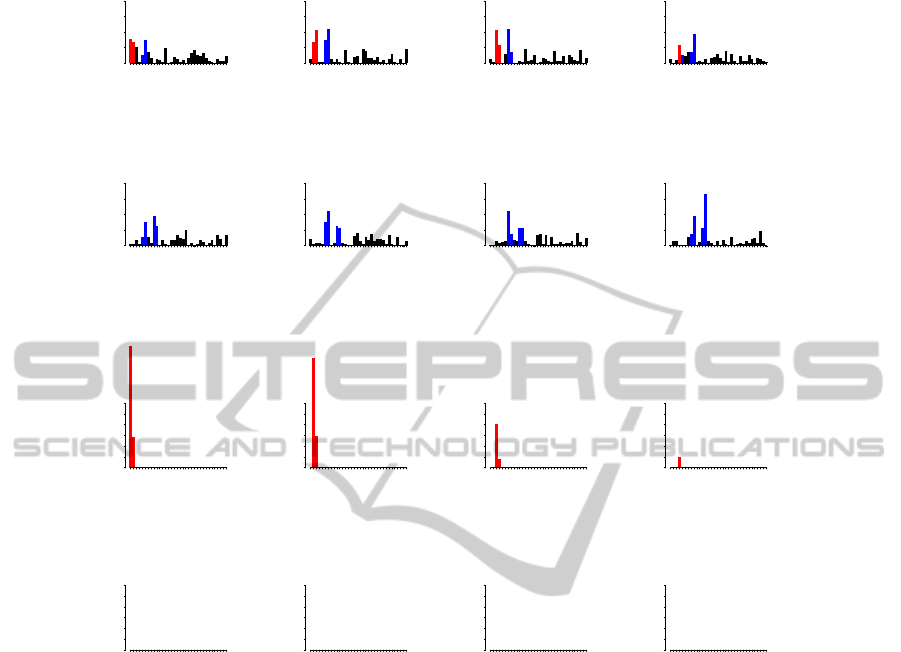
Figure 2: T
2
score contribution plot from PLS vs. contribution plot from our target-aware method for experiments with a
basic linear model. Contributions for all variables are shown for the first 8 test samples. Correct relevant contributors are
shown with red bars. Other contributors are shown with blue bars. For the first three outliers there are 2 relevant contributors,
the fourth outlier has only 1 relevant contributor, and the other four groups have none.
4 EXPERIMENTS
The only existing competitive method for supervised
outlier ranking and contribution estimation is a PLS
contribution plot analysis which is widely used in sta-
tistical process control (along with more traditional
PCA). However, linear methods can be ineffective for
nonlinear high-dimensional data with many noisy or
irrelevant attributes. We illustrate the limitations of
PLS on several experimental scenarios that are very
similar to actual problems that are encountered in
manufacturing applications. Typical data have very
few relevant inputs and/or contributors for an outlier,
even when the total number of inputs can range from
several hundreds to tens of thousands. Therefore,
consider similar, representative scenarios in our ex-
periments, but with the pragmatic advantage that the
ground truth is known. From a linear model built with
PLS we can obtain two scores: SPE (distance from
the model that is computed in the same way as PCA)
and T
2
(modified with Y-loadings). It is worthy to
mention that the SPE score is useless for distinguish-
ing influential/non-influential outliers or contribution
analysis as it does not use Y-loadings.
TARGET-AWARE ANOMALY DETECTION AND DIAGNOSIS
19

396 431 466 501 536 571
PLS SPE score
samples
score
0 2 4 6 8 10
396 431 466 501 536 571
PLS T^2 score
samples
score
0 1 2 3 4
(a) SPE, T
2
scores from PLS.
396 431 466 501 536 571
GBT outlier score
samples
score
0 10 20 30 40
396 431 466 501 536 571
GBT prediction errors
samples
score
0.0 1.0 2.0 3.0
(b) Outlier scores from our target-aware method and prediction errors on the samples (for reference).
Figure 3: SPE and T
2
score plots from PLS vs. our target-aware method for a linear model with 100 noise variables. Samples
with relevant contributors (influential outliers) and non-influential outliers are shown with red and blue bars, respectively.
Each outlier has one contributor.
4.1 Linear Data with Noise
Reference data are simulated from 34 independent
attributes with 500 samples (rows). Each is nor-
mally distributed with mean zero and standard devi-
ation one. The four first attributes are relevant predic-
tors, with the target y = x
1
+ 0.5x
2
+ 0.3x
3
+ 0.15x
4
.
The other 30 attributes are irrelevant. We added 100
test samples generated from the same distribution, in
which we create 20 anomalies. Anomaly i has values
of attributes x
i
, x
i+1
, x
i+4
, x
i+5
equal to 5. Therefore,
the first three outliers have 2 relevant and 2 irrelevant
contributors, the fourth outlier has 1 relevant contribu-
tor, and the other outliers have 0 relevant contributors
(all 4 contributors irrelevant) to the target. The targets
for these additional samples are generated from the
same linear function of relevant variables. For PLS
we used two latent components as suggested by cross
validation based on the explained y-variance. (The
two components explained 98% of the y variance.) A
GBT model was built with 700 trees, shrinkage rate
= 0.01, tree depth = 4, and each tree used 60% sub-
sampling. The least squares loss function was em-
ployed.
Figure 1 shows the PLS SPE and T
2
plots for 50
(last) training samples and all testing samples for this
example, compared to the GBT outlier scores plot.
Figure 1 shows that PLS cannot distinguish the
influential and non-influential outliers. Actually it
does not even separate the two last influential out-
liers, while the target-aware outlier score plot gener-
ates the correct results. All four influential outliers are
ICINCO 2011 - 8th International Conference on Informatics in Control, Automation and Robotics
20

450 475 500 525 550 575 600
PLS SPE score
samples
score
0 2 4 6 8 10
450 475 500 525 550 575 600
PLS T^2 score
samples
score
0 1 2 3 4
(a) SPE, T
2
scores from PLS.
450 475 500 525 550 575 600
GBT outlier score
samples
score
0 20 40 60
450 475 500 525 550 575 600
GBT prediction errors
samples
score
0 5 15 25
(b) Outlier scores from our target-aware method and prediction error on the samples (for reference).
Figure 4: SPE and T
2
score plots from PLS vs. our target-aware method for nonlinear data. Samples with relevant contributors
(influential outliers) and non-influential outliers shown with red and blue bars, respectively.
detected, without false alarms. Furthermore, the in-
fluential outliers are correctly ranked and their scores
are higher than the scores for the non-influential out-
liers and the normal samples (non-outliers). Also,
the figure shows that the target-aware outlier scores
are very well correlated to prediction errors for the
corresponding samples. Although, as mentioned pre-
viously, the prediction errors are assumed to not be
available at the time of these diagnostics. The PLS T
2
plot cannot even separate outliers from non-outliers.
While the SPE plot can separate in this case, below
we have the slightly modified version of this example
where it fails too.
Figure 2 shows plots of PLS T
2
contribution
scores and target-aware outlier score contributions for
the first 16 test samples.
Again PLS does not correctly rank and separate
the relevant and irrelevant contributors. The target-
aware outlier scores correctly detect and rank both the
outliers and the contributing attributes with respect to
their effect on the target.
However, when the number of noise attributes in-
crease and the outliers do not deviate much from zero,
the SPE and T
2
plots may not detect them at all. Con-
sider a simplified version of the above linear example
with 100 noise attributes, and each i-th outlier is cre-
ated by setting x
i
= 5. Figure 3) shows PLS SPE and
T
2
plots vs the target-aware scores plot for this exam-
ple.
It can be seen that now SPE cannot readily iden-
tify outliers, although their scores are slightly above
average, and T
2
shows only the single most influential
outlier.
4.2 Nonlinear Data
Next we consider a similar example with the target a
nonlinear function of inputs–a quadratic target func-
tion y = x
2
1
+0.5x
2
2
+0.3x
2
3
+0.15x
2
4
. All other settings
were similar to the previous experiment, except we
used four latent components for PLS (again as sug-
gested by a 10-fold cross-validation model error plot).
Figure 4 shows PLS SPE and T
2
plots for 35 (last)
training samples and all test samples for this example,
TARGET-AWARE ANOMALY DETECTION AND DIAGNOSIS
21
1 6 12 19 26 33
obs501
variables
PLS T^2 contr
0.00 0.10 0.20
1 6 12 19 26 33
obs502
variables
PLS T^2 contr
0.00 0.10 0.20
1 6 12 19 26 33
obs503
variables
PLS T^2 contr
0.00 0.10 0.20
1 6 12 19 26 33
obs504
variables
PLS T^2 contr
0.00 0.10 0.20
1 6 12 19 26 33
obs505
variables
PLS T^2 contr
0.00 0.10 0.20
1 6 12 19 26 33
obs506
variables
PLS T^2 contr
0.00 0.10 0.20
1 6 12 19 26 33
obs507
variables
PLS T^2 contr
0.00 0.10 0.20
1 6 12 19 26 33
obs508
variables
PLS T^2 contr
0.00 0.10 0.20
(a) Contribution from PLS T
2
scores.
1 6 12 19 26 33
obs501
variables
GBT contr
0 4 8 12
1 6 12 19 26 33
obs502
variables
GBT contr
0 4 8 12
1 6 12 19 26 33
obs503
variables
GBT contr
0 4 8 12
1 6 12 19 26 33
obs504
variables
GBT contr
0 4 8 12
1 6 12 19 26 33
obs505
variables
GBT contr
0 4 8 12
1 6 12 19 26 33
obs506
variables
GBT contr
0 4 8 12
1 6 12 19 26 33
obs507
variables
GBT contr
0 4 8 12
1 6 12 19 26 33
obs508
variables
GBT contr
0 4 8 12
(b) Contributions from target-aware outlier scores.
Figure 5: T
2
score contribution plot from PLS vs. contribution plot for our target-aware method for nonlinear data. Contri-
butions for all variables are shown for the first 8 test samples. Correct relevant contributors are shown with red bars. Other
contributors are shown with blue bars. For the first 3 outliers there are 2 relevant contributors, the fourth outlier has only 1
relevant contributor, and the other four groups have none.
along with our target-aware outlier scores plot.
Figure 4 indicates that PLS cannot distinguish
the influential and non-influential outliers (actually it
does not separate even the last two influential out-
liers), while the target-awareoutlier scores plot gener-
ates the correct results. It shows that all four influen-
tial outliers are correctly detected and ranked, without
false alarms. Also it can be seen that the target-aware
outlier scores are well correlated to prediction errors
for corresponding samples. The PLS T
2
plot fails to
separate even outliers from non-outliers.
Figure 5 shows plots of PLS T
2
contribution
scores and target-aware outlier score contributions for
the first 16 test samples.
Again PLS fails to correctly rank and separate rel-
evant and irrelevant contributors. Still, target-aware
outlier scores correctly rank the outliers and the con-
tributing attributes with respect to their effect on the
target.
5 CONCLUSIONS
The target-aware anomaly detection and associated
contribution problem is introduced to the machine
learning community and a solution for complex data
from modern systems is described. Newoutlier scores
and contributions are developed, and thresholds (de-
ICINCO 2011 - 8th International Conference on Informatics in Control, Automation and Robotics
22

rived from baselines obtained from target permuta-
tions) are used to filter non-influential outliers and
normal samples. The target-aware paradigm uses
target-labeled data for training, but the diagnostics are
calculated before the corresponding target attribute
value is available (to meet the conditions for pro-
cess control applications). The ensemble model al-
lows us to deal with complex interactions in predic-
tor space and local data structures. Linear methods
based on principal components often fail to detect
outliers and/or contributors in anomaly detection, es-
pecially in the presence of noise. The linear meth-
ods are also sensitive to scaling. Furthermore, linear
methods rarely work when the target is a non-linear
function of the inputs. Furthermore, methods such as
partial least squares often fail to rank the contributors
correctly and fail to separate relevant from irrelevant
contributors. When the number of irrelevant variables
increases it even can fail to identify influential outliers
on relevant predictors. The proposed method works
equally well for linear and non-linear cases in terms
of diagnostics. Our method can correctly rank out-
liers with respect to their effect on the target, rank at-
tributes that contribute to an outlier score, and filter
non-influential and normal sample. It is insensitive
to noise and ranks outliers and contributors for a data
sample using a fast, robust, nonparametric technique.
ACKNOWLEDGEMENTS
This research was partially supported by ONR grant
N00014-09-1-0656. We wish to thank anonymous
referees for comments that improved this work.
REFERENCES
Angelov, P., Giglio, V., Guardiola, C., Lughofer, E., and
Luj´an, J. (2006). An approach to model-based fault
detection in industrial measurement systems with ap-
plication to engine test benches. Measurement Science
and Technology, 17:1809.
Borisov, A., Eruhimov, V., and Tuv, E. (2006). Tree-
based ensembles with dynamic soft feature selection.
In Guyon, I., Gunn, S., Nikravesh, M., and Zadeh,
L., editors, Feature Extraction Foundations and Ap-
plications: Studies in Fuzziness and Soft Computing.
Springer.
Breiman, L., Friedman, J., Olshen, R., and Stone, C. (1984).
Classification and Regression Trees. Wadsworth, Bel-
mont, MA.
Chandola, V., Banerjee, A., and Kumar, V. (2009).
Anomaly detection: A survey. ACM Computing Sur-
veys (CSUR), 41(3):15.
Chiang, L., Russell, E., and Braatz, R. (2001). Fault de-
tection and diagnosis in industrial systems. Springer
Verlag.
Efendic, H., Schrempf, A., and Del Re, L. (2003). Data
based fault isolation in complex measurement sys-
tems using models on demand. In Proceedings of the
5th IFAC-Safeprocess 2003, IFAC, pages 1149–1154.
ACM.
Ergon, R. (2004). Informative pls score-loading plots for
process understanding and monitoring. Journal of
Process Control, 14(6):889–897.
Filev, D. and Tseng, F. (2006). Novelty detection based
machine health prognostics. In Evolving Fuzzy Sys-
tems, 2006 International Symposium on, pages 193–
199. IEEE.
Friedman, J. H. (2001). Greedy function approximation: A
gradient boosting machine. The Annals of Statistics,
29(5):1189–1232.
Hastie, T., Tibshirani, R., and Friedman, J. (2001). The
Elements of Statistical Learning. Springer.
Hodge, V. J. and Austin, J. (2004). A survey of outlier de-
tection methodologies. Artificial Intelligence Review,
22:85–126.
Hotelling, H. (1947). Multivariate quality control-
illustrated by the air testing of sample bombsights.
In Eisenhart, C., Hastay, M., and Wallis, W., edi-
tors, Techniques of Statistical Analysis, pages 111–
184. McGraw-Hill, New York.
Lughofer, E. and Guardioler, C. (2008). On-line fault detec-
tion with data-driven evolving fuzzy models. Control
and Intelligent Systems, 36(4):307–317.
Miller, P., Swanson, R., and Heckler, C. (1998). Contri-
bution plots: A missing link in multivariate quality
control. Applied Mathematics and Computer Science,
8(4):775–792.
Runger, G., Alt, F., and Montgomery, D. (1996). Con-
tributors to a Multivariate Statistical Process Control
Chart Signal. Communications in Statistics–Theory
and Methods, 25(10):2203–2213.
Wold, S., Sjostrom, M., and Eriksson, L. (2001). PLS-
regression: a basic tool of chemometrics. Chemo-
metrics and intelligent laboratory systems, 58(2):109–
130.
TARGET-AWARE ANOMALY DETECTION AND DIAGNOSIS
23
