
WAYPOINT GUIDANCE BASED PLANAR PATH FOLLOWING
AND OBSTACLE AVOIDANCE OF AUTONOMOUS
UNDERWATER VEHICLE
Saravanakumar S. and Asokan T.
Robotics Laboratory, Department of Engineering Design, IIT Madras, Chennai, India
Keywords: Underwater robotics, Path planning, AUV, Obstacle avoidance, Potential field, Line-of-sight.
Abstract: This paper presents waypoint guidance based planar path following and obstacle avoidance for Autonomous
Underwater Vehicles (AUV). Guidance through waypoints by line-of-sight (LOS) method and artificial
potential field method (APFM) are used to develop the algorithm. Both LOS and PFM are simple and
computationally inexpensive and can be used for real-time implementation. The basic LOS method has been
modified for reference heading correction with a distance threshold in order to achieve minimal calculation
for heading correction and smoother vehicle turn during course change at waypoints. An improved potential
field method is also proposed for better obstacle avoidance for the AUV. Few points are taken from the path
generated by the waypoint guidance and given as via points for the obstacle avoidance algorithm. The
proposed algorithm basically follows the improved LOS method when there is no obstacle along the
vehicle’s path and switches to APFM when any obstacle is detected. The details of the algorithm and
simulation results are presented.
1 INTRODUCTION
Applications of AUV have seen rapid growth in the
last few decades. Guidance, navigation and control
(GNC) are important to an autonomous vehicle’s
mission success and utility. However the
effectiveness of AUV is still limited by the precision
and accuracy of guidance schemes. The main
purpose of the guidance is to receive the target
related information from the navigation system and
generate references for the vehicle control system so
as the vehicle can move through a set of way points
as per the given sequence. It may be a time variant
trajectory tracking or time invariant path following.
Guidance system also includes sophisticated features
like obstacle avoidance, minimum time navigation,
fuel optimization and weather routing (Fossen,
1994). Several guidance laws such as waypoint
guidance by LOS, vision based guidance, Lyapunav
based guidance, guidance using chemical signals and
magnetometers, proportional navigation guidance,
and electromagnetic guidance are being used for
developing guidance strategies. Waypoint guidance
by LOS is one the most widely used method for
AUV due to its simplicity and computational
advantages. But it has a major drawback of
undesirable control energy consumption due to
overshoot during course change at waypoints
(Naeem et al., 2003). Fossen et al. (2003) presented
a LOS method that uses straight lines and circular
arcs in order to get smooth transition between two
consecutive waypoints. Though the vehicle makes a
better turn, its path is far away if a U-turn is made at
a waypoint thus missing the waypoint. Bakaric et al.
(2004) proposed a technique to avoid the missed
waypoint and the overshoot issues by considering
the next waypoint before the current waypoint is
reached. In this method, the vehicle calculates the
heading correction from the starting point itself
though it is not essentially needed if the vehicle is
too far away from the target point. Obstacle
avoidance algorithm can also be incorporated in the
design of waypoint guidance systems (Fossen,
2002). Road map, cell decomposition, optimal
control and potential field methods are used for
developing obstacle avoidance schemes. Artificial
potential field method for obstacle avoidance was
initially proposed by Khatib (1985). Koren and
Bronstein (1992) discussed the potential field
method and their inherent limitations. Potential field
191
S. S. and T. A..
WAYPOINT GUIDANCE BASED PLANAR PATH FOLLOWING AND OBSTACLE AVOIDANCE OF AUTONOMOUS UNDERWATER VEHICLE.
DOI: 10.5220/0003531401910198
In Proceedings of the 8th International Conference on Informatics in Control, Automation and Robotics (ICINCO-2011), pages 191-198
ISBN: 978-989-8425-75-1
Copyright
c
2011 SCITEPRESS (Science and Technology Publications, Lda.)
method is mostly used for on-line obstacle
avoidance (Al-Sultan and Aliyu, 1996). Ge and Cui
(2000) presented a new artificial potential field
method for mobile robot path planning in order to
avoid goal non reachable with obstacle nearby
(GNRON) problem. Ding Fu-guang et al. (2005)
developed a path planning method using virtual
potential field concept for AUV. In most cases, the
potential field methods are used for mobile robots
and the potential of an obstacle is calculated at only
one point. Hence an improved guidance strategy is
required for better path following and obstacle
avoidance for an AUV. In this paper, we propose an
improved path following and obstacle avoidance
strategy to address this. The waypoint guidance by
LOS is modified by locating a distance threshold
point in the direction of the waypoints. The vehicle
can take any course angle correction only in between
these threshold points and the waypoints. This
reduces the computation of heading correction.
Similarly, the obstacle avoidance can be improved
by discretizing both the periphery of the obstacle
and an arc of radius around the AUV into many
points. The potential fields due to each point on an
obstacle can be calculated and integrated to obtain a
strengthened potential field for that particular
obstacle.
The rest of the paper is organized in four
sections. In Section 2, the guidance based path
following algorithm is described by modifying the
waypoint guidance by LOS guidance law. Section 3
presents the development of obstacle avoidance
algorithm using artificial potential field method.
Here, the environment is taken as local minima free.
Section 4 consists of simulation results for path
planning and obstacle avoidance of an AUV.
Finally, the conclusion and future work are given in
section 5.
2 WAYPOINT GUIDANCE BY
LINE OF SIGHT
We can define the LOS in terms of a desired heading
angle (Fossen, 1994) as
,tan
1
⎟
⎟
⎠
⎞
⎜
⎜
⎝
⎛
−
−
=
−
xx
yy
i
i
r
ψ
(1)
where (
,
) for
(
=1…
)
is the given set of
waypoints. When the vehicle lies within the circle of
acceptance with a radius
around the waypoint
(
,
), that is if the vehicle location V(, )
satisfies:
=(
−)
+(
−)
)≤
, (2)
where
is the distance between vehicle position
and the current waypoint. Then the next waypoint
(
,
) can be selected. The radius of circle
of acceptance is taken as 2L, where L is the length
of the vehicle. The basic LOS algorithm has a
disadvantage that the vehicle will not turn smoothly
during course change since the reference heading is
calculated only with respect to the current waypoint.
In order to achieve smoother turn at the waypoints,
the waypoint guidance by LOS is modified by
making some corrections on the reference heading
determined from the basic LOS guidance law. The
algorithm can be explained as follows. Let (, )
is the starting point, (, )is the goal point,
(
,
) and (
,
) are the current and
next waypoints as shown in Figure 1. Now the
vehicle is located at (, ). A distance threshold
point
(
,
) is located before the current
waypoint in the direction of current waypoint.
Similarly another threshold point
(
,
) is
located after the current waypoint in the direction of
next waypoint. The distance threshold is taken as
10L. This is an adjustable constant and it is
sufficient even if any sharp U-turn is needed. Let
(
,
) and (
,
) are the auxiliary points at
a distance
in the direction of next and current
waypoints. The coordinates of the point
are given
as (Bakaric et al., 2004):
()
iAi
ii
ii
iAi
ii
ii
ii
ii
oiAi
yy
yy
xx
xx
yyif
yy
xx
yy
yy
−
⎟
⎟
⎠
⎞
⎜
⎜
⎝
⎛
−
−
+=
≠
⎟
⎟
⎠
⎞
⎜
⎜
⎝
⎛
−
−
+
−
+=
+
+
+
+
+
+
1
1
1
2
1
1
1
)(
1
)sgn(
ρ
(3)
Similarly,
()
iAi
ii
ii
iAi
ii
ii
ii
ii
oiAi
xx
xx
yy
yy
xxif
xx
yy
xx
xx
−
⎟
⎟
⎠
⎞
⎜
⎜
⎝
⎛
−
−
+=
≠
⎟
⎟
⎠
⎞
⎜
⎜
⎝
⎛
−
−
+
−
+=
+
+
+
+
+
+
1
1
1
2
1
1
1
)(
1
)sgn(
ρ
(4)
The coordinates of the point
can be given as
()
iBi
ii
ii
iBi
ii
ii
ii
ii
oiBi
yy
yy
xx
xx
yyif
yy
xx
yy
yy
−
⎟
⎟
⎠
⎞
⎜
⎜
⎝
⎛
−
−
+=
≠
⎟
⎟
⎠
⎞
⎜
⎜
⎝
⎛
−
−
+
−
+=
−
−
−
−
−
−
1
1
1
2
1
1
1
)(
1
)sgn(
ρ
(5)
ICINCO 2011 - 8th International Conference on Informatics in Control, Automation and Robotics
192
Similarly,
()
iBi
ii
ii
iBi
ii
ii
ii
ii
oiBi
xx
xx
yy
yy
xxif
xx
yy
xx
xx
−
⎟
⎟
⎠
⎞
⎜
⎜
⎝
⎛
−
−
+=
≠
⎟
⎟
⎠
⎞
⎜
⎜
⎝
⎛
−
−
+
−
+=
−
−
−
−
−
−
1
1
1
2
1
1
1
)(
1
)sgn(
ρ
(6)
The distance between vehicle and the auxiliary
points can be calculated as,
22
2
22
2
)()(
)()(
yyxx
d
yyxx
d
BiBi
Bi
AiAi
Ai
−+−=
−+−=
(7)
The normalized difference between the auxiliary and
the distance threshold points can be given as,
,
o
CBiBi
Bi
o
PiAi
Ai
dd
dd
ρ
ε
ρ
ε
−
=
−
=
(8)
where
Ai
ε
and
Bi
ε
are the normalized difference
factors and
CBi
d
is the distance between the vehicle
position and the distance threshold point
(
,
).
If both the current and next waypoints are in the
same direction, the normalized difference factor
becomes 1, and no heading correction is required. If
the next waypoint lies in the direction of current
waypoint, this factor is near to 1. Whenever a sharp
turn is needed, this factor gets the value near to -1.
The heading correction
c
ψ
is zero at the distance
threshold points and at the waypoints. A linear curve
fitting is done in order to find the different values for
heading correction. The values are taken as distance
factor and angle factors. The sign of the heading
correction
sc
ψ
can be determined as
{}
{}
)).(()).((sgn
)).(()).((sgn
xxyyyyxx
xxyyyyxx
iBiiBisc
iAiiAisc
−−−−−=
−−−−−=
ψ
ψ
(9)
The heading correction
c
ψ
can be calculated as
)().().(
)().().(
BiAPiBdscc
AiAPiAdscc
fdf
fdf
εψ
ψ
ε
ψ
ψ
=
=
(10)
where the distant factors
)(
PiAd
df
,
)(
PiBd
df
and
the angle factors
)(),(
BiBAiA
ff
ε
ε
are determined
using Figure 2, 3 and 4. Finally the desired heading
is calculated as (Bakaric et al., 2004)
crd
ψ
ψ
ψ
+=
(11)
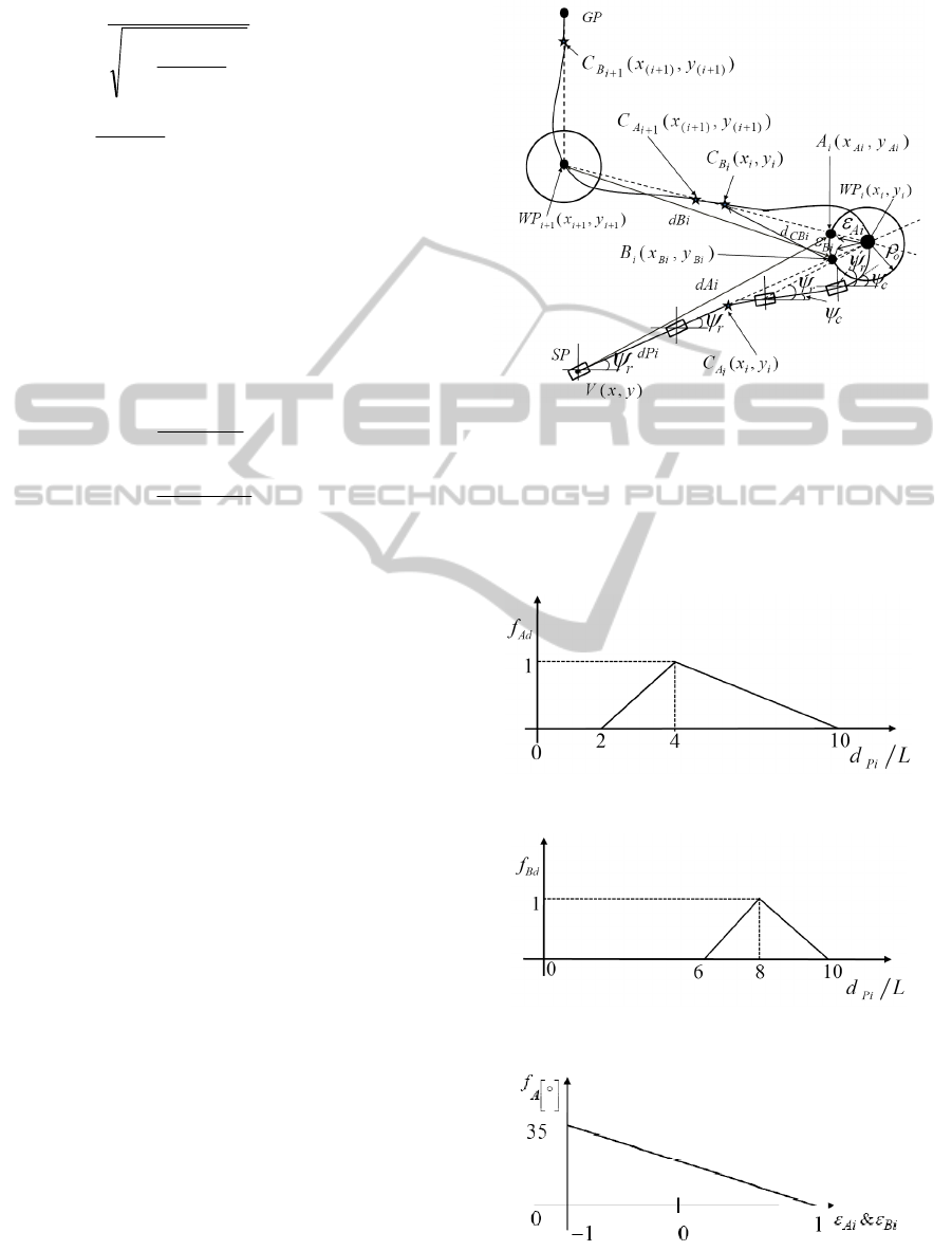
Figure 1: Calculation of heading correction for smooth
turn during course change at waypoints.
This heading correction is calculated between the
points
,
and the current waypoints. In this
way the LOS guidance algorithm is improved to turn
the vehicle smoothly at both sides of the waypoints.
Figure 2: Distance factor for the auxiliary point A
i
.
Figure 3: Distance factor for the auxiliary point B
i
.
Figure 4: Angle factors for calculating heading correction.
WAYPOINT GUIDANCE BASED PLANAR PATH FOLLOWING AND OBSTACLE AVOIDANCE OF
AUTONOMOUS UNDERWATER VEHICLE
193
3 OBSTACLE AVOIDANCE BY
POTENTIAL FIELD METHOD
The objective of the obstacle avoidance algorithm is
to find an obstacle free path by avoiding the
obstacles so that the vehicle can reach the desired
goal position without collision. The artificial
potential field method is used for developing the
obstacle avoidance algorithm. The main idea of this
potential field method is to generate attraction and
repulsion potentials for the target and the obstacles.
The target has an attraction potential and the
obstacles have repulsion potentials. By determining
the point at which the minimum potential exists
among the total potentials, the vehicle can be
commanded to that point. The total potential can be
calculated by integrating the attraction and repulsive
potentials at few points around the periphery of the
vehicle.
The obstacle avoidance algorithm has been
developed in 2D space based on the artificial
potential field method with static obstacles. The
following assumptions are made for the
implementation of the algorithm.
The vehicle is assumed to be flat-fish type
AUV.
The obstacles are assumed as static and they
are in circular shape of various sizes
Forward looking sonar data is used for
developing the control algorithm.
The vehicle cannot move in sideways.
The vehicle is neutrally buoyant and there are
no external disturbances
The following steps give the methodology of the
obstacle avoidance algorithm.
Discretize the arc of radius r around the AUV
into N points (
:1=1,2,…) over a range of
interest defined by
, and
. (Refer Figure. (5))
Compute the attractive potential
att
U
at these
points. The attraction influence tends to pull the
vehicle towards the target position. The most
commonly used attractive potential field is of the
form (Ge and Cui, 2000):
()
()
,
2
1
)(
2
i
a
i
att
dqU
ξ
=
(12)
where
()
aia
qqd
i
−=
is the distance between
i
q
th
point around the vehicle and the goal point
a
q
.
ξ
is
an adjustable constant.
Obtain the location and size of the obstacle from
the sonar data and discretize its periphery into K
points (
:1= 1,2,…).
Compute the repulsive potential
obs
U
at
i
q
due
to the obstacle point
j
p
. The repulsive potential
fields are intended to generate a high potential
around the obstacle, such that the gradient flow
points away from the obstacle. The repulsion
influence tends to push the vehicle away from the
obstacles. The repulsive potential at
i
q
due to the
obstacle point
j
p
is given as (Ge and Cui, 2000)
(13)
where
()
j
io
pqd
ji
−=
,
, is the distance between
i
q
th
point around the vehicle and
j
p
th
point on the
periphery of the obstacle,
t
d
is the influence
distance,
η
is an adjustable constant.
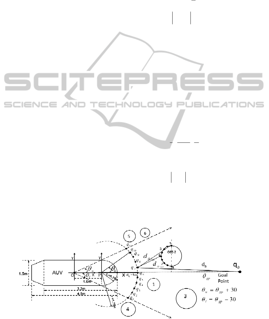
Figure 5: Methodology for the implementation of 2D obstacle avoidance algorithm.
()
()
()
()
()
⎪
⎪
⎪
⎪
⎩
⎪
⎪
⎪
⎪
⎨
⎧
>
≤
⎟
⎟
⎟
⎠
⎞
⎜
⎜
⎜
⎝
⎛
−
=
to
to
a
to
obs
ddif
ddifd
dd
qU
ji
ji
i
ji
ji
,
,
,
,
,0
,
11
2
1
)(
2
2
η
ICINCO 2011 - 8th International Conference on Informatics in Control, Automation and Robotics
194
Compute the actual repulsive potential
rep
U
at
i
q
due to the obstacle
()
()
)()(
1
,
qUqU
K
j
obsrep
ji
i
∑
=
=
(14)
Compute the total potential
tot
U
at each point
around the vehicle. The total potential at a point
around the vehicle is represented as a sum of
attractive potential and all the repulsive potentials.
Here the repulsive potential results from the
superposition of the individual repulsive potentials
generated by the obstacles.
()
()
()
∑
=
+=
R
m
repatttot
qUqUqU
mi
i
i
1
)()()(
,
(15)
where m=1,2…,R. R is the number of obstacles,
()
)(qU
i
att
represents the attractive potential and
()
)(
,
qU
mi
rep
represents the repulsive potentials
generated by the obstacle m. The above steps can be
represented in a single equation as,
()
()
()
()
()
()
()
⎪
⎪
⎪
⎪
⎩
⎪
⎪
⎪
⎪
⎨
⎧
>
≤
⎟
⎟
⎟
⎠
⎞
⎜
⎜
⎜
⎝
⎛
−
+=
∑∑
==
to
to
a
to
K
j
R
m
atttot
ddif
ddifd
dd
qUqU
mji
mji
i
mji
i
i
,,
,,
,,
,0
,
11
2
1
)(
2
2
11
η
(16)
where i=1,2,…,N; j=1,2,…,K and m=1,2,…,R. In
this way, obtain the total potential for all the points
around the vehicle and predict the next one step
ahead by determining the minimum potential
tot
U
min
.
)min(
min tottot
UU =
(17)
Represent the minimum potential point in
Cartesian space.
Command the vehicle to the position calculated
in the previous step.
Repeat the above steps till the goal is reached.
The above steps can be explained using Figure 5 as
an example. Let the starting, goal positions are given
and the obstacle information are received from
sensor. Initially the vehicle is at the start position. In
this methodology, the vehicle is always aimed
towards the target. In order to determine the next
position, an arc around the AUV is discretized into
eleven (N=11) equidistant points. The way of
selecting few points around the vehicle is shown in
Figure 5. The angle (
θ
) between the starting point
and goal point is calculated in the horizontal plane.
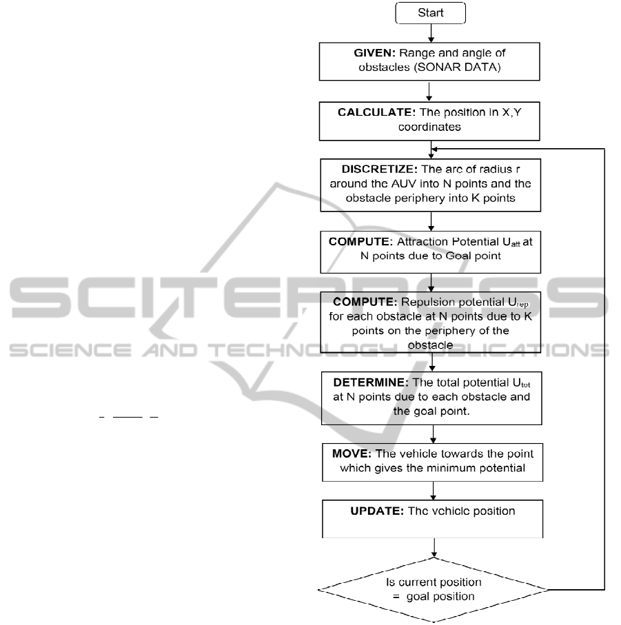
Figure 6: Flow chart for the obstacle avoidance algorithm.
A range of interest is determined by the distance
influence threshold and the angles
)(
u
θ
θ
+
and
)(
l
θ
θ
−
, where
°
= 30
u
θ
and
°
= 30
l
θ
are the upper
and lower limit angles and they can be adjusted in
order to define the obstacle region. The obstacles are
considered only if they are within this region. The
obstacles 2, 3 and 4 are existing in this region and
the rests are out of the region. Now there are 1 one-
step ahead points with radial distance of two meter
around the vehicle and 15 degrees apart. (i.e.,
h
θ
= -
75, -60, -45, -30, -15, 0, 15, 30, 45, 60, 75 degrees).
So each point is having a heading angle of 15
WAYPOINT GUIDANCE BASED PLANAR PATH FOLLOWING AND OBSTACLE AVOIDANCE OF
AUTONOMOUS UNDERWATER VEHICLE
195
degree. The points (
i
q
) on the semicircle in terms
of Cartesian co-ordinates can be represented as
,sin
cos
hi
hi
ry
rx
θ
θ
=
=
(18)
where r =r
v
+d
q
, (r
v
=radius of the AUV nose (0.75m),
d
q
=radial distance of the points
i
q
around the
vehicle). These points are used to “predict” the next
one step ahead. The distance (
a
d
) between a point
on the arc (
i
q
) and the goal point is measured and
the attractive potential is calculated using eq. (12).
To calculate the repulsive potential, sixteen (K=16)
points are taken on the periphery of the obstacle 2.
Using eq. (13), the repulsive potential is calculated
at each point on the arc (
i
q
) by measuring the
distance (
o
d
) between this point and the point (
j
p
)
on the obstacle 2. The actual repulsion potential due
to the obstacle 2 at the point on the arc is the sum of
individual potential calculated by using the eq. (13).
In this way, the actual potentials for other obstacles
within the region of interest are also calculated.
Since
tot
U
is the sum of the attractive and repulsive
potentials, we need to add all the actual repulsion
potentials due to the obstacles 1, 2, and 3 at the point
(
i
q
) and this has to be added with attractive
potential corresponding to the point on the arc (
i
q
).
Once the total potentials are computed for N points,
then the vehicle is moved to the point at which
tot
U
has minimum value. The algorithm is shown as
flowchart in Figure 6.
4 SIMULATION RESULTS
In order to illustrate the performance of the way
point guidance based path planning algorithm,
simulations are carried out by taking the length of
the vehicle as L=4.5 m and the desired forward
speed
= 2 m/s. The path of the modified
waypoint guidance by LOS method and the basic
LOS are shown in Figure 7. The minimum distance
between starting point, waypoints and goal point can
be fixed by adjusting the distance threshold value.
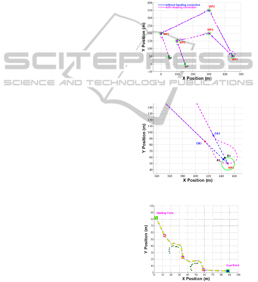
From Figure 7, it can be seen that the vehicle takes a
smooth turn at the waypoints using the modified
waypoint guidance by LOS method. A close-up
view of the course change at waypoint-3 is shown in
Figure 8. The vehicle computes for heading
correction only between the distance threshold and
waypoints though the line showing the path between
waypoint and goal point is not via the threshold
point C
B
. It can be seen that there is a smooth
transition exists at waypoints and also passes
through it. The simulations are carried out for
obstacle avoidance algorithm and the results have
been shown in Figure 9 and 10. Here the obstacles
are considered along the path of the vehicle in a
manner such a way that there will be no local
minima.
Figure 7: Waypoint guidance with and without heading
correction.
Figure 8: Close-up view of the modified waypoint
guidance by LOS at waypoint 3.
Figure 9: 2D Obstacle avoidance of AUV with circular
obstacles of same size.
ICINCO 2011 - 8th International Conference on Informatics in Control, Automation and Robotics
196
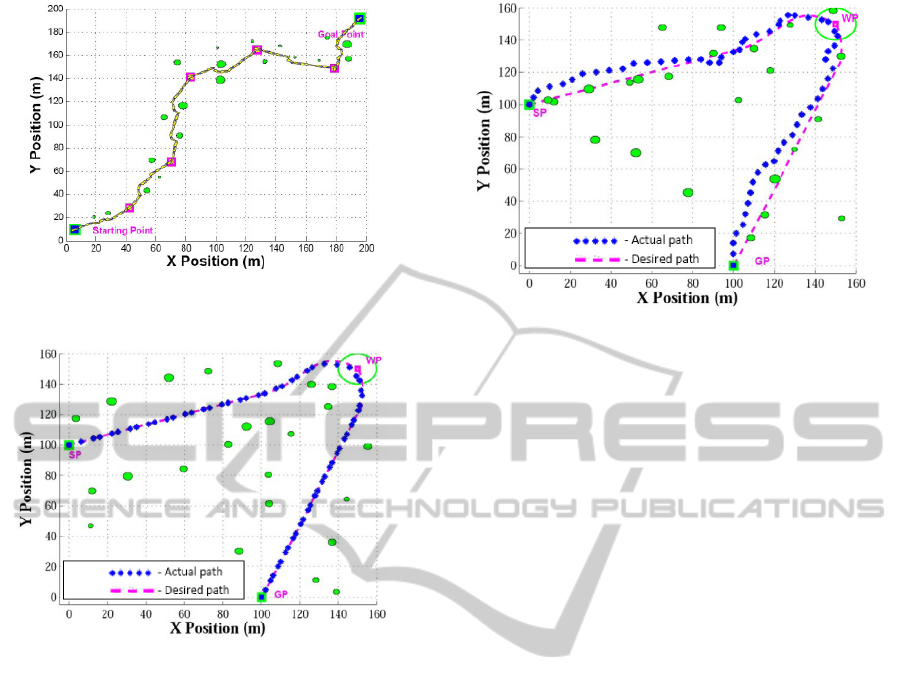
Figure 10: 2D Obstacle avoidance of AUV with circular
obstacles of various sizes.
Figure 11: Obstacle avoidance with improved waypoint
guidance data – No obstacle in the desired path.
In order to showcase the position and orientation of
the vehicle during maneuvering the vehicle is
considered as a flat fish type AUV. It has been
observed that the vehicle is able to reach the desired
goal position successfully after avoiding the
obstacles by maintaining the orientation. Few points
are taken from the path generated by the improved
waypoint guidance. These points are given as
waypoints for the obstacle avoidance algorithm. The
corresponding results are shown in Figure 11 and 12.
It has been observed that the obstacle avoidance
algorithm follows the path if there is no obstacle in
the path. In case of any obstacles found, it avoids the
obstacles and follows the path.
5 CONCLUSIONS AND FUTURE
WORK
A waypoint guidance based path following is
developed by improving the basic LOS method for
smooth turn during course change at waypoints.
Simulation results show that it is possible to achieve
Figure 12: Obstacle avoidance for the obstacles of various
sizes in the desired path with the improved waypoint
guidance data.
a better and smooth transition though a sharp turn is
required and computation for heading correction is
needed for minimal distance only. These path points
can be used to generate a trajectory and can be used
for better vehicle control so that the vehicle will
follow the trajectory. This algorithm also eliminates
the problem of changing the waypoints by the
mission planner in order to avoid a sharp turn. An
obstacle avoidance algorithm has been developed by
adding some improvements to the artificial potential
field method. The desired path generated by the
waypoint guidance algorithm can be given to the
obstacle avoidance algorithm. This algorithm helps
the vehicle to avoid the obstacles and reach the
target successfully. Both the algorithms are simple
and appropriate for real-time implementation. These
algorithms are being improved to address the issues
of local minima as well as dynamic environments.
Hardware in the loop (HIL) simulations will be
carried out in order to validate these algorithms for
real time implementation. The results will be
presented in the near future.
REFERENCES
Fossen, T. I., 1994. Guidance and control of ocean
vehicles,
John Wiley & Sons Ltd., Chichester.
Fossen, T. I., 2002. Marine Control Systems: Guidance,
Navigation and Control of Ships, Rigs and Underwater
Vehicles, Marine Cybernetics AS, Trondheim,
Norway.
Fossen, T. I., Breivik, M., and Skjetne, R., 2003. Line-of-
Sight path following of underactuated marine craft. In
IFAC MCMC'03,
Proceedings of the IFAC MCMC'03,
Girona, Spain.
Khatib, O., 1985. Real-time obstacle avoidance for
manipulators and mobile robots.
In IEEE International
WAYPOINT GUIDANCE BASED PLANAR PATH FOLLOWING AND OBSTACLE AVOIDANCE OF
AUTONOMOUS UNDERWATER VEHICLE
197

Conference on Robotics and Automation, pp. 500-505.
Naeem, W., Sutton, R., Ahmad, S. M., Burns, R. S., 2003.
A Review of Guidance Laws Applicable to Unmanned
Underwater Vehicles.
In Journal of Navigation,
Vol.56, pp. 15-29.
Bakaric, V., Vukic, Z., and Antonic, R., 2004. Improved
basic planar algorithm of vehicle guidance through
waypoints by the line of sight. In Proceedings IEEE
1st International Symposium on control,
Communications and Signal Processing
, pp. 541-544.
Koren, Y., Borenstein, J., 1992. Potential field methods
and their inherent limitations for mobile robot
navigation,
In Proceedings of the IEEE conference on
Robotics and Automation
, pp. 1398-1404.
Al-Sultan, K. S., Aliyu, M. D. S., 1996. A new potential
field based algorithm for path planning. In Journal of
Intelligence and Robotic Systems
, Vol.17, pp. 265-
282.
Ge, S. S., Cui, Y. J., 2000. New potential functions for
mobile robot path planning,
In IEEE transactions on
Robotics and Automation
, Vol.16, No.5 pp. 615-620.
Ding Fu-guang, Jiao Peng, Bian Xin-qian and Wang
Hong-jian, 2005. AUV local path planning based on
virtual potential,
In Proceedings of the IEEE
International conference on Mechatronics &
Automation
, Niagara Falls, Canada.
ICINCO 2011 - 8th International Conference on Informatics in Control, Automation and Robotics
198
