
OPTIMIZATION LEARNING METHOD FOR DISCRETE
PROCESS CONTROL
Ewa Dudek-Dyduch and Edyta Kucharska
Institute of Automatics, AGH University of Science and Technology, al. Mickiewicza 30, PL 30-059 Krakow, Poland
Keywords: Discrete Manufacturing Processes Control, Optimization Method, Learning Algorithm.
Abstract: The aim of the paper is to present a novel conception of the optimization method for discrete manufacturing
processes control. This method uses gathering information during the search process and a sophisticated
structure of local optimization task. It is a learning method of a special type. A general formal model of a
vast class of discrete manufacturing processes (DMP) is given. The model is a basis for learning algorithms.
To illustrate the presented ideas, the scheduling algorithm for a special NP-hard problem is given.
1 INTRODUCTION
The control of Discrete Manufacturing Process
(DMP) lies in determining the manner of performing
a certain set of jobs under restrictions referring to
machines/devices, resources, energy, time,
transportation possibilities, order of operation
performing and others. Most of control algorithms
are approximate (heuristic) due to NP-hardness of
the optimization problems. Within the frame of
artificial intelligence, one attempts at both formal
elucidation of heuristic algorithm ideas and giving
some rules for creating them (metaheuristics)
(Dudek-Dyduch and Fuchs-Seliger, 1993),
(Dudek-Dyduch and Dyduch, 1988), (Pearl, 1988),
and (Rajedran, 1994). The paper ties in with this
direction of research. It deals with formal modeling
of discrete manufacturing/production processes and
its applications for control/planning algorithms. It
presents the development of ideas given in
(Dudek-Dyduch, 2000). Its aim is twofold:
To present a novel heuristic method that uses
a sophisticated local optimization and
gathering information during consecutive
search iterations (learning method);
To present an intelligent search algorithm
based on the method for a certain NP-hard
scheduling problem, namely a scheduling
problem with state depended retooling.
The paper uses the formal model based on
the special type of the multistage decision process
given below.
2 FORMAL MODEL OF DMP
Simulation aimed at scheduling any DMP consists in
determining a sequence of process states and the
related time instances. The new state and its time
instant depend on the previous state and the decision
that has been realized (taken) then. The decision
determines the job to be performed, resources,
transport unit, etc. Manufacturing processes belong
to the larger class of discrete processes, namely
discrete deterministic processes (DDP). The formal
model of DDP given in (Dudek-Dyduch, 1990),
(Dudek-Dyduch, 1992), and (Dudek-Dyduch, 1993)
will be adopted here for DMP.
Definition 1. A discrete manufacturing/pro-
duction process (DMP) is a process that is defined
by the sextuple DMP=(U, S, s
0
, f, S
N
, S
G
) where U is
a set of control decisions or control signals, S=X×T
is a set named a set of generalized states, X is a set
of proper states, T
+
{0} is a subset of non
negative real numbers representing the time
instants, f:U×S
S is a partial function called
a transition function, (it does not have to be
determined for all elements of the set U×S),
s
0
=(x
0
,t
0
), S
N
S, S
G
S are respectively: an initial
generalized state, a set of not admissible generalized
states, and a set of goal generalized states, i.e.
the states in which we want the process to take place
at the end.
It can be noticed, that DMP corresponds to some
multistage decision processes.
24
Dudek-Dyduch E. and Kucharska E..
OPTIMIZATION LEARNING METHOD FOR DISCRETE PROCESS CONTROL.
DOI: 10.5220/0003532400240033
In Proceedings of the 8th International Conference on Informatics in Control, Automation and Robotics (ICINCO-2011), pages 24-33
ISBN: 978-989-8425-74-4
Copyright
c
2011 SCITEPRESS (Science and Technology Publications, Lda.)

The transition function is defined by means of
two functions, f=(f
x
,f
t
) where f
x
:
U×X×T
X
determines the next state, f
t
:
U×X×T
T determines
the next time instant. It is assumed that the
difference
t =f
t
(u, x, t)-t has a value that is both
finite and positive.
Thus, as a result of the decision u that is taken or
realized at the proper state x and the moment t, the
state of the process changes for x’=f
x
(u, x, t) that is
observed at the moment t’=f
t
(u, x, t)=t+
t.
Because not all decisions defined formally make
sense in certain situations, the transition function f is
defined as a partial one. As a result, all limitations
concerning the control decisions in a given state s
can be defined in a convenient way by means of so-
called sets of possible decisions U
p
(s), and defined
as: U
p
(s)={u
U: (u, s)
Dom f}.
At the same time, a DMP is represented by a set
of its trajectories that starts from the initial state s
0
. It
is assumed that no state of a trajectory, apart from
the last one, may belong to the set S
N
or has
an empty set of possible decisions. Only a trajectory
that ends in the set of goal states is admissible.
The control sequence determining an admissible
trajectory is an admissible control sequence
(decision sequence). The task of optimization lies in
the fact of finding such an admissible decision
sequence ũ that would minimize a certain criterion
Q.
In the most general case, sets U and X may be
presented as a Cartesian product U=U
1
×U
2
×...×U
m
,
X=X
1
×X
2
×...×X
n
i.e. u=(u
1
,u
2
,...,u
m
), x=(x
1
,x
2
,...,x
n
).
There are no limitations imposed on the sets; in
particular they do not have to be numerical. Thus
values of particular co-ordinates of a state may be
names of elements (symbols) as well as some
objects (e.g. finite set, sequence etc.). Particular u
i
represent separate decisions that must or may be
taken at the same time. The sets S
N
, S
F
, and U
p
are
formally defined with the use of logical formulae.
Therefore, the complete model constitutes
a specialized form of a knowledge-based model
(logic-algebraic model). According to its structure,
the knowledge on DMP is represented by coded
information on U, S, s
0
, f, S
N
, S
G
. Function f may be
defined by means of a procedure or by means of
IF..THEN rules. The basic structure of DMP (def.1)
is usually created on the basis of process technology
description. Based on additional expert knowledge
(or analysis of DMP) subsets of states can be
differentiated, for which best decisions or some
decision choice rules R (control rules) are known.
3 OPTIMIZATION LEARNING
METHOD
The method of solution search with information
gathering is a significant development of the method
presented in papers (Dudek-Dyduch, 1990),
(Dudek-Dyduch, 2000), which generates subsequent
process trajectories with the use of previously
obtained and analyzed solutions (admissible and
non-admissible trajectories) so as to generate
improved solutions.
The method uses local optimization tasks.
The task lies in the choice of such a decision among
the set of possibilities in the given state U
p
(s), for
which the value of a specially constructed local
criterion is the lowest. The form of the local
criterion and its parameters are modified in
the process of solution search.
The local criterion consists of three parts and is
created in the following way. The first part concerns
the value of the global index of quality for the
generated trajectory. It consists of the increase of the
quality index resulting from the realization of the
considered decision and the value related to the
estimation of the quality index for the final
trajectory section, which follows the possible
realization of the considered decision. This part of
the criterion is suitable for problems, whose quality
criterion is additively separable and monotonically
ascending along the trajectory (Dudek-Dyduch,
1990).
The second part consists of components related
to additional limitations or requirements.
The components estimate the distance in the state
space between the state in which the considered
decision has been taken and the states belonging to
the set of non-admissible states S
N
, as well as
unfavorable states or distinguished favorable states.
Since the results of the decision are known no
further than for one step ahead, it is necessary to
introduce the “measure of distance” in the set of
states, which will aid to define this distance. For that
purpose, any semimetrics can be applied. As we
know, semimetrics, represented here as
, differs
from metrics in that it does not have to fulfill
the condition
(a,b)=0
a=b.
The third part includes components responsible
for the preference of certain types of decisions
resulting from problem analysis. The basic form of
the criterion q(u,x,t) can be then represented as
follows:
q(u,x,t)=
Q(u,x,t)+̂Q(u,x,t)+
+a
1
1
(u,x,t)+…+a
i
i
(u,x,t)+…+a
n
n
(u,x,t)+
+b
1
1
(u,x,t)+…+b
j
j
(u,x,t)+…+ b
n
n
(u,x,t)
(1)
OPTIMIZATION LEARNING METHOD FOR DISCRETE PROCESS CONTROL
25

where:
Q(u,x,t) - increase of the quality index value
as a result of decision u, undertaken in
the state s=(x,t);
ˆQ(u,x,t) - estimation of the quality index value
for the final trajectory section after
the decision u has been realized;
i
(u,x,t) - component reflecting additional
limitations or additional requirements in
the space of states, i=1,2,...,n;
a
i
- coefficient, which defines the weight of i-th
component
i
(u,x,t) in the criterion q(u,x,t);
j
(u,x,t) - component responsible for
the preference of certain types of decisions,
j=1,2,...,m;
b
j
- coefficient, which defines the weight of j-th
component responsibles for the preference of
particular decision types.
The significance of particular local criterion
components may vary. The more significant a given
component is, the higher value is of its coefficient. It
is difficult to define optimal weights a priori. They
depend both on the considered optimization problem
as well as the input date for the particular
optimization task (instance). The knowledge
collected in the course of experiments may be used
to verify these coefficients. On the other hand,
coefficient values established for the best trajectory
represent aggregated knowledge obtained in
the course of experiments.
The presented method consists in the
consecutive construction of whole trajectories,
whilst their generation always begins from the initial
state s
0
=(x
0
,t
0
). For each generated trajectory, both
admissible and non-admissible, its final
characteristics is remembered and then used in
further calculations. The method is characterized by
the following features:
A trajectory sequence is generated; each
trajectory is analyzed, which provides
information about the DMP taken control;
Based on the analysis of so far generated
whole trajectories, it is possible to modify
coefficients used in local optimization or
change the form of local optimization
criterion when generating a new trajectory;
In the course of trajectory creation,
the subsequent state of the process is being
analyzed and it is possible to modify the form
or/and parameters used in local optimization.
4 SCHEDULING PROBLEM
WITH STATE DEPENDED
RETOOLING
To illustrate the application of the presented method,
let us consider the following real life scheduling
problem that takes place during scheduling
preparatory works in mines. The set of headings in
the mine must be driven in order to render the
exploitation field accessible. The headings form a
net formally, represented by a nonoriented
multigraph G=(W,C,P) where the set of branches C
and the set of nodes W represent the set of headings
and the set of heading crossings respectively, and
relation P
(W×C×W) determines connections
between the headings (a partial order between the
headings).
There are two kinds of driving machines that
differ in efficiency, cost of driving and necessity of
transport. Machines of the first kind (set M1) are
more effective but the cost of driving by means of
them is much higher than for the second kind (set
M2). Additionally, the first kind of machines must
be transported when driving starts from another
heading crossing than the one in which the machine
is, while the second type of machines need no
transport. Driving a heading cannot be interrupted
before its completion and can be done only by one
machine at a time.
There are given due dates for some of
the headings. They result from the formerly prepared
plan of field exploitation. One must determine
the order of heading driving and the machine by
means of which each heading should be driven so
that the total cost of driving is minimal and each
heading complete before its due date.
There are given: lengths of the headings dl(c),
efficiency of both kinds of machines V
Dr(m)
(driving
length per time unit), cost of a length unit driven for
both kinds of machines, cost of the time unit waiting
for both kinds of machines, speed of machine
transport V
Tr(m)
and transport cost per a length unit.
The problem is NP-hard (Kucharska, 2006).
NP-hardness of the problem justifies the application
of approximate (heuristic) algorithms. A role of
a machine transport corresponds to retooling during
a manufacturing process, but the time needed for
a transport of a machine depends on the process state
while retooling does not.
ICINCO 2011 - 8th International Conference on Informatics in Control, Automation and Robotics
26

4.1 Formal Model of Problem
The process state at any instant t is defined as
a vector x=(x
0
,x
1
,x
2
,...,x
|M|
), where M=M1
M2.
A coordinate x
0
describes a set of heading (branch)
that has been driven to the moment t. The other
coordinates x
m
describes state of the m-th machine,
where m=1,2,...,|M|.
A structure of the machine state is as follows:
x
m
=(p,
,
)
(2)
where:
p
C
{0} - represents the number of
the heading assigned to the m-th machine to
drive for p
C or no assignment for
the machine for p=0 (if the machine is not
assigned to a heading, i.e. the machine
remains idle at the crossing w);
W - the number of the crossing (node),
where the machine is located (if it is not
assigned to any heading, i.e. p=0) or
the number of the node, in which it finishes
driving the assigned heading c (information
about movement direction of the machine);
[0,∞) - the length of the route that remains to
reach the node
=w by the m-th machine,
whilst
=0 means, that the machine is in node
w,
(0,dl(c)) means that the machine is
driving a heading, and the value of
is the
length that remains for the given heading c to
be finished, whilst
>dl(c) means that the
machine is being transported to the heading,
the value
is the sum of the length of heading
c and the length of the route until the
transportation is finished.
A state s=(x,t) belongs to the set of
non-admissible states if there is a heading whose
driving is not complete yet and its due date is earlier
than t. The definition S
N
is as follows:
S
N
={s=(x,t): (
c
C, c
x
0
)
d(c) < t}
(3)
where d(c) denotes the due date for the heading c.
A state s=(x,t) is a goal if all the headings have
been driven. The definition of the set of goal states
S
G
is as follows:
S
G
={s=(x,t) : s
S
N
(
c
C, c
x
0
)}
(4)
A decision determines the headings that should
be started at the moment t, machines which drive,
machines that should be transported, headings along
which machines are to be transported and machines
that should wait. Thus, the decision u=(u
1
,u
2
,...,u
|M|
)
where the co-ordinate u
m
refers to the m-th machine
and u
m
=C
{0}. u
m
=0 denotes continuation of
the previous machine operations (continuation of
driving with possible transport or further stopover).
u
m
=c denotes the number of heading c that is
assigned to be driven by machine m. As a result of
this decision, the machine starts driving the heading
c or is transported from the current location to
the node of the heading c, to which
the transportation route defined in the state s is
the shortest. This route is computed by the Ford’s
algorithm (a polynomial one).
Obviously, not all decisions can be taken in
the state (x,t). The decision u(x,t) must belong to
the set of possible (reasonable) decisions Up(x,t).
For example, a decision u
m
=c is possible only when
the c-th heading is neither being driven nor complete
and is available, i.e. there is a way to transport
machine to the one of the heading crossing adjacent
to the c-th heading or machine is standing in the one
of the heading crossings adjacent to the c-th heading.
Moreover, in the given state s=(x,t), to each
machine waiting in the node w, (it has not assigned
a heading to perform), we can assign an available
heading or it can be decided that it should continue
to wait. However, each machine which has been
previously assigned a heading and is currently
driving it or it is being transported to that heading,
can be only assigned to continue the current activity.
Also, none of the headings can be assigned to more
than one machine. The complete definition of the set
of the possible decision U
p
(x,t) will be omitted here
because it is not necessary to explain the idea of
the learning method.
Based on the current state s=(x,t) and
the decision u taken in this state, the subsequent
state (x’,t’)=f(u,x,t) is generated by means of
the transition function f. The transition function is
defined for each possible decision u(s)
U
p
(s).
Firstly, it is necessary to determine the moment
t’ when the subsequent state occurs, that is
the nearest moment in which at least one machine
will finish driving a heading. For that purpose, t
m
time of completion of the realized task needs to be
calculated for each machine. The subsequent state
will occur in the moment t’=t+
t, where
t equals
the lowest value of the established set of t
m
.
Once the moment t’ is known, it is possible to
determine the proper state of the process at the time.
The first coordinate x
0
of the proper state, that is the
set of completed headings, is increased by
OPTIMIZATION LEARNING METHOD FOR DISCRETE PROCESS CONTROL
27

Table 1: Particular parameters of the coordinate of the new machine state.
for the decision to continue the activity of the machine u
m
= 0:
ttfor
ttforp
p
m
m
0
'
’=
2
10,
0),(max
max,
0),(max
min
'
)(
)(
)(
)(
)(
MmfortV
Mmfor
V
cdl
tVt
V
cdl
V
mDr
mTr
mDr
mTr
mTr
for the decision to assign a new task to the machine u
m
= c:
ttfor
ttforc
p
m
m
0
'
’ =w
k
(c)
2)(
10,
),(
max,
),(
min)(),(
'
)(
)(
min
)(
)(
min
)(min
MmfortVcdl
Mmfor
V
cmr
tVt
V
cmr
Vcdlcmr
mDr
mTr
mDr
mTr
mTr
the number of headings whose driving has been
finished in the moment t’.
Afterwards, the values of subsequent coordinates
in the new state are determined x’
m
=(p’,
’,
’), for
m=1,2...|M|, which represent the states of particular
machines.
Particular parameters of the coordinate of
the new machine state are determined in the way
described in Table 1, where w
k
(c) is the node
adjacent to the heading c, in which the machine will
finish driving, and |r
min
(m,c)| is the length of the
shortest transportation route to the heading c for the
machine m.
4.2 Learning Algorithm
The algorithm based on the learning method consists
in generating consecutive trajectories. Each of them
is generated with the use of the specially designed
local optimization task and then is analyzed.
The information gained as a result of the analysis is
used in order to modify the local optimization task
for the next trajectory, i.e. for the next simulation
experiment. This approach is treated as a learning
without a teacher.
In the course of trajectory generation in each
state of the process, a decision is taken for which
the value of the local criterion is the lowest.
The local criterion takes into account a component
connected with cost of work, a component
connected with necessity for trajectory to omit
the states of set S
N
and a component for preferring
some decisions.
The first components is a sum of
Q(u,x,t) and
ˆQ(u,x,t) where
Q(u,x,t) denotes the increase of
work cost as a result of realizing decision u and
ˆQ(u,x,t) the estimate of the cost of finishing the set
of headings matching the final section of
the trajectory after the decision u has been realized.
The second component
1
(u,x,t)=E(u,x,t),
connected with the necessity for the trajectory to
omit the states of set S
N
, is defined by means of
a semimetrics.
The third component is aimed at reduction of
machine idleness time. Since the model considers
the possibility that the machines will stand idle in
certain cases, it seems purposeful to prefer decisions
which will engage all machines to for most of
the time. It is therefore necessary to reduce
the probability of selecting the decision about
machine stopover when headings are available for
driving and machines could be used for work. This
may be realized by using an additional auxiliary
ICINCO 2011 - 8th International Conference on Informatics in Control, Automation and Robotics
28

criterion
1
(u,x,t)=F(u,x,t), which takes into
consideration penalty for a decision about a stopover
in the case of a machine which could have started
work.
Thus, the local criterion is of the form:
q(u,x,t)=
Q(u,x,t)+̂Q(u,x,t)+
+a
1
E(u,x,t)+b
1
F(u,x,t)
(5)
where
a
1
, b
1
are weights of particular
components.
In the course of trajectory generation, the local
optimization task may be changed. Problem
analysis reveals that the moment all headings with
due dates are already finished, it is advisable to use
only cheaper machines. Formally, this corresponds
to the limitation of the set of possible decisions
Up(s).
Moreover, it is no longer necessary to apply
the
component
E(u,x,t)
in the local criterion.
The modified form of the criterion can be then
represented as follows:
q(u,x,t)=
Q(u,x,t)+̂Q(u,x,t)+ b
1
F(u,x,t)
(6)
In order to select a decision in the given state s, it
is necessary to generate and verify the entire set of
possible decisions in the considered state U
p
(s). For
each decision u
k
, it is necessary to determine
the state the system would reach after realizing it.
Such a potentially consecutive state of the process
will be represented as s
p_k
=(x
p_k
,t
p_k
).
Afterwards, the criterion components are
calculated. The increase of cost
Q(u
k
,x,t) is the sum
of costs resulting from the activities of particular
machines in the period of time t
p_k
-t. The estimate of
the cost of the final trajectory section ˆQ(u
k
,x,t) can
be determined in a number of ways. One of these is
to establish the summary cost of finishing previously
undertaken decisions, whose realization has not been
completed yet, and the cost of a certain relaxed task,
realized in the cheapest way. Taking into
consideration that the estimate should take place
with the lowest number of calculations, relaxation
has been proposed which would include omitting
temporal limitations and the assuming the least
expensive procedure for finishing the remaining
headings; this would involve using the least
expensive machines.
The component of the local criterion E(u
k
,x,t)
uses the value of the estimated “distance” between
the state s
p_k
, and the set of inadmissible states.
The distance is estimated with the help of
semimetrics
(s,S
N
)=min{
(s,s’): s’
S
N
}.
Assuming that the speed of transporting
the “fastest” machine is significantly higher than its
speed of performance, and this one in turn
significantly exceeds the speed of performance of
the remaining machines, it is possible to omit
the time of transporting the fastest machine. For
the sake of simplicity, let us assume that there is one
fastest machine.
One of the methods of determining
the component E(u
k
,x,t) is to calculate, for each not
realized and not assigned heading c with due date,
the time reserve rt
c
(s
p_k
).
Taking into consideration these assumptions,
the time reserve is defined by the following formula:
rt
c
(s
p
k
)=d(c)-t
p
k
-
(c)-t
end
(7)
where:
d(c) - due date for the heading c;
(c) - time necessary to drive heading c and all
the headings situated along the shortest route
from the heading c to the so-called realized
area in the given state, by the fastest machine;
t
end
- time necessary to finalize the current
activity of the fastest machine
.
The parameters t
end
and
(c) results for following
situations:
a) “the fastest” machine may continue
the previously assigned task to drive another
heading.
b) heading c may be inaccessible and it might
be necessary to drive the shortest route to this spot
from the realized area, involving already excavated
headings as well as those assigned for excavation
together with relevant crossings. For the period of
time when the fastest machine finishes
the excavation of the previously assigned heading,
a fragment of this distance may be excavated by the
fastest of the remaining machines. When the heading
is accessible the time equals to the time of
excavating the length of the heading with the fastest
machine.
Finally, the component estimating the influence
of time limitations assumes the following form:
_
_
_
min ( ) 0
1
(,,)
min ( ) 0
min ( )
cpk
k
cpk
cpk
for rt s
Eu xt
for rt s
rt s
(8)
As a result, the decision to be taken, from the set
of considered decisions, is the one for which the
subsequent state is most distant from the set of
non-admissible states.
The shape of the local criterion component
F(u
k
,x,t) in certain cases should make it purposeful
to prefer decisions which will engage all machines
OPTIMIZATION LEARNING METHOD FOR DISCRETE PROCESS CONTROL
29

for most of the time. It is therefore necessary to
reduce the probability of selecting the decision about
machine stopover when headings are available for
driving and machines could be used for work. For
that purpose, a penalty may be imposed for the
stopover of each machine that could potentially start
driving an available heading. The proposed form of
F(u
k
,x,t) is the following:
F(u
k
,x,t)=P
i
waitin
g
(9)
where:
P - denotes the penalty for machine stopover,
(calculated for the decision about stopover
when there are still headings available for
work);
i
waiting
- the number of machines that are
supposed to remain idle as a result of such
a decision.
The values a
1
and b
1
are respectively coefficients
defining the weight of particular components of
the local criterion q(u,x,t) and reflect current
knowledge about controls, whilst their values change
in the course of calculations. The higher the weight
of a given parameter, the higher its value.
The weights depend both on the considered
optimization problem as well as input data for
the particular optimization task (instance).
Coefficient values, as well as their mutual
proportions are not known nor can they be
calculated a priori.
The knowledge gained in the course of
experiments may be used to change weight values. If
the generated trajectory is non-admissible, then for
the subsequent trajectory, the value of weight a
1
should be increased; which means the increase of
the weight of the component estimating the distance
from the set of non-admissible states and/or
the increase of weight b
1
value, which would result
in lower probability of machine stopover.
Whereas, if the generated trajectory is
admissible, then for the subsequent trajectory the
values of this coefficients may be decreased.
4.3 Experiments
The aim of conducted experiments was to verify the
effectiveness of applying the components E(u,x,t)
and F(u,x,t) in the local criterion.
The research was conducted for the set of 10
heading networks. Each network is represented by
a planar graph, in which the vertex degrees equal
from 1 to 4. The lengths of headings are numbers
from the range [19, 120]. The number of headings
with due dates is approximately 25% of all headings.
The parameters of heading networks used in
simulation experiments are given in Table 2.
Also, two examples of network are presented in
Figure 1.
Two machines are used to perform the task
during our experiments, one of the first type and one
of the second type. Parameters for both types of
machines are given in the Table 3.
The effectiveness of component E(u,x,t) for each
network was tested by constructing 40 trajectories
with the changing value of coefficient a
1
and zero
value of coefficient b
1
.
Table 2: The heading network parameters.
Parameter GI-1a GI-1b GI-2
GI-3 GII-4 GII-5a GII-5b GII-6 GII-7 GII-8
Number of heading
20 20 20
20 24 27 27 29 67 68
Number of heading crossing
18 18 18
18 20 20 20 20 50 50
Length of the shortest
heading
20 20 22
19 30 30 30 30 30 30
Length of the longest
heading
109 109 106
120 81.59 107.52 107.52 94.75 114.65 111.95
Sum of the length of
the headings
1008 1008 1010 1066 1364.45 1863.07 1863.07 1869.88 4579.11 4607.81
Number of heading with
deadline
5 5 5
5 5 5 5 5 18 16
Minimum deadline
55 60 55
55 60 70 100 50 80 80
Maximum deadline
70 60 70
70 100 150 100 100 320 200
ICINCO 2011 - 8th International Conference on Informatics in Control, Automation and Robotics
30
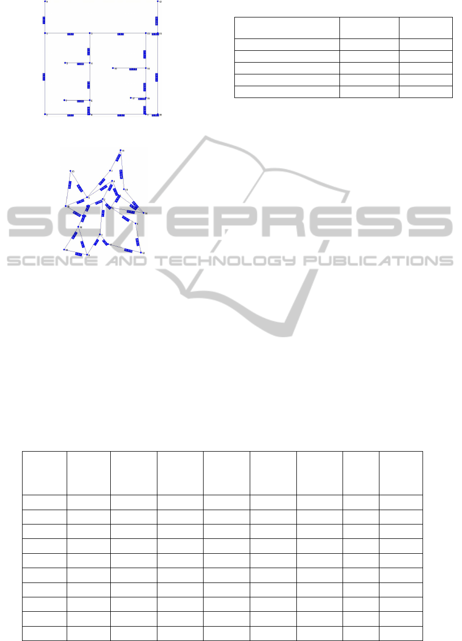
Figure 1a: Example of heading network - GI-1a.
Figure 1b: Example of heading network - GII-5.
Table 4 presents results for one of the tested
networks, i.e. for network GII-4.
The time reserve refers to the time that remains after
a given heading has been driven until the due date,
whilst the minus value means that the due date has
been exceeded. The symbol ”*” means that heading
driving has not commenced because the trajectory
reached a non-admissible state. Based on
the obtained results, it can be concluded that
increasing the value of E(u,x,t) increases
the probability of obtaining an admissible solution.
Table 3: Parameters of the machines.
Parameter Machine of
M1 type
Machine
of M2 type
Efficiency [m/h]
10.0 5.0
Transport speed [m/h]
100.0 unspecified
Driving cost [$/h]
200.0 50.0
Transport cost [$/h]
100.0 0.0
Waiting cost [$/h]
30.0 5.0
When the component E(u,x,t) was omitted,
an admissible solution was not found.
Table 5 presents in columns the best obtained
total cost at changeable value of coefficient b
1
,
responsible for the weight of component F(u,x,t) in
the local criterion. In most cases, the increase of
weight of this component resulted in increased total
costs, but at the same time the probability of finding
an admissible solution was higher. Moreover, in
some cases, the use of this component resulted in
decreased total costs of performing work. A lot of
this experiments have been conducted, they are
presented in (Kucharska, 2006). Unfortunately, they
must be omitted here because the limited length of
the paper.
The experiments have confirmed effectiveness
of the use of the component F(u,x,t).
To evaluate the effectiveness of the proposed
algorithm one has compared the obtained results
with the optimal solution. A complete review
algorithm for all considered heading network has
been applied. To reduce calculations, the generation
of each trajectory was interrupted when the lower
estimate of its cost in a given state was greater than
the best found solution.
Table 4: The effectiveness of applying parameter E(u,x,t) for the network GII-4.
Coeff. a
1
Total
cost
Time
reserve of
head. 4
Time
reserve of
head. 9
Time
reserve of
head. 12
Time
reserve of
head. 16
Time
reserve of
head. 22
Min.
reserve
Average
reserve
0 - 7.40 * * * * - -
1 - 12.90 * * * * - -
50 - 12.90 * -0.62 * * - -
5000 - 12.90 * -2.84 * * - -
7500 22887.64 12.90 4.02 7.68 5.15 11.64 4.02 8.28
25000 23153.10 13.18 32.10 48.01 1.46 2.67 1.46 19.48
50000 23359.93 12.90 21.73 48.01 38.90 30.34 12.90 30.38
75000 23204.35 25.18 19.42 48.01 20.54 25.59 19.42 27.75
500000 23027.78 27.47 20.13 19.71 40.06 29.18 19.71 27.31
2500000 23084.25 27.47 20.13 19.71 36.57 37.53 19.71 28.28
OPTIMIZATION LEARNING METHOD FOR DISCRETE PROCESS CONTROL
31
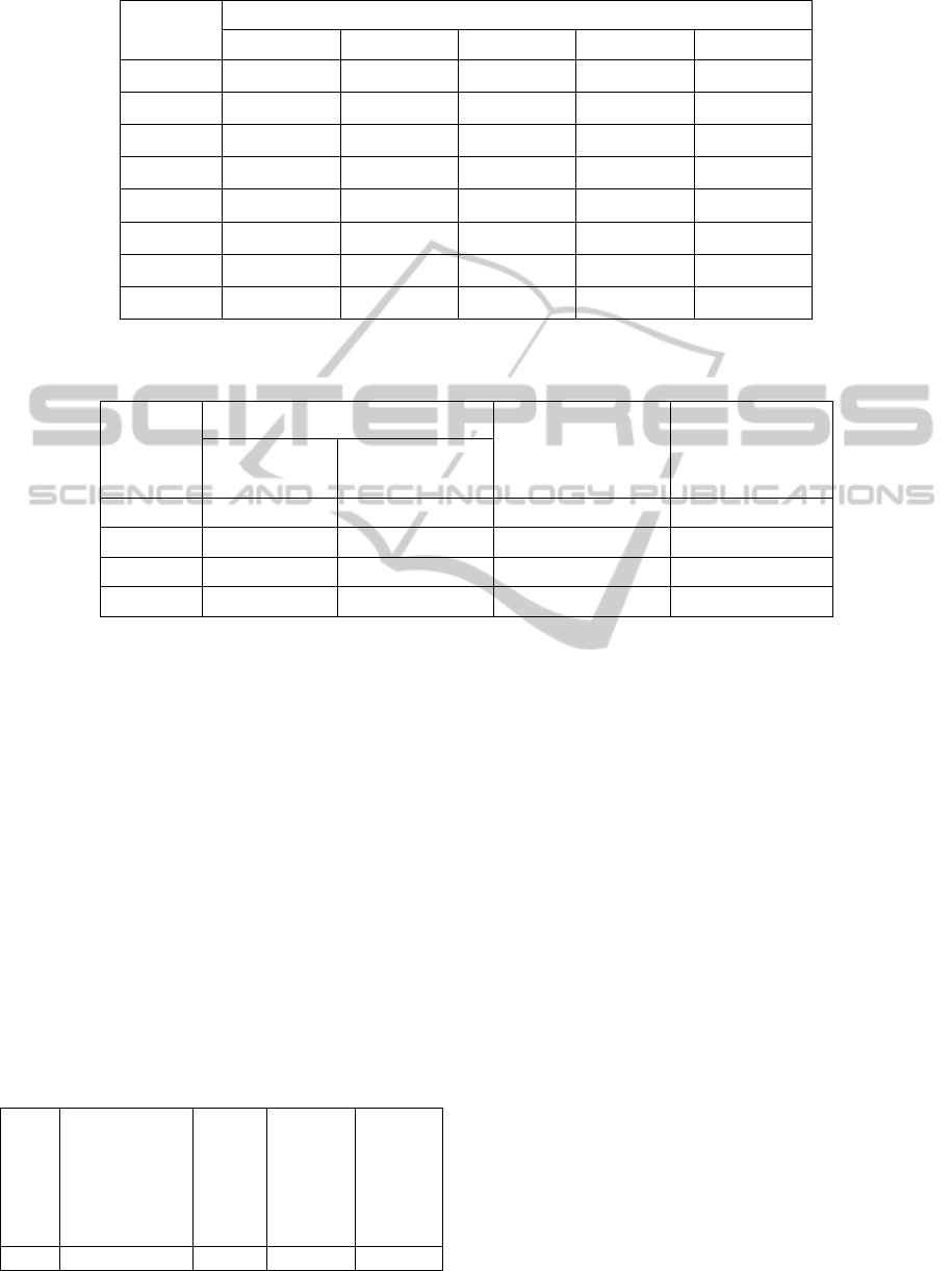
Table 5: Effectiveness of applying component F(u,x,t).
Network
Best found cost
b
1
=0 b
1
=0,5 b
1
=1 b
1
=2 b
1
=5
GI-1a 17026.90 17026.90 17249.10 16922.00 16922.00
GI-2 * * * 17284.10 17284.10
GI-3 16359.90 16359.90 16359.90 16359.90 16359.90
GII-4 22665.17 22665.17 22667.89 22667.89 22667.89
GII-5a 30982.02 30946.33 31004.27 31004.27 31004.27
GII-5b 30888.34 30888.34 31139.72 31139.72 31139.72
GII-6 30662.32 30675.19 30675.19 30675.19 30675.19
GII-7 77428.92 77717.02 77288.44 77717.02 77717.02
Table 7: Comparison of results from the solution obtained by a complete review of the algorithm for which the calculations
were interrupted.
Network
Review algorithm
Best cost founded by
learning algorithm
Percentage
difference of cost
time to stop
calculation
best found cost
GI-1a 43h 48min 16480,00 16922.00 2,68%
GI-3 43h 41min 17448,90 16359.90 -6,24%
GII-4 44h 3min 23132,40 22665.17 -2,01%
GII-6 43h 38min 31142,54 30662.32 -1,54%
The lower bound was calculated as the sum of
the cost of the current part of trajectory and a cost
estimation of remaining part.
Optimal solution was found only for network
GI-2. In other cases, the calculations were
interrupted after more than 2 days. Only for four
networks an admissible solution has been found,
while for the other networks an acceptable solution
has not been found during 2 days.
The comparison between the optimal cost with
the best found cost is presented in Table 6. Error of
found solution is also given. It can be noticed that
the proposed learning algorithm has found very good
solution (almost optimal). It should be point out also
that the its calculation time was very short (a several
seconds). While the exact algorithm needs very long
time (over 40 hours).
Table 6: Comparison of results from the optimal solution.
Net-
work
Time for the
optimal
solution
Optimal
cost
The best
cost
found by
the
proposed
algorithm
Error of
found
solution
GI-2 43h 43min 59s 16524.40 17284.10 4.59%
The comparison of the learning algorithm results
with solution obtained by complete review algorithm
after over 40 hour are presented in Table 7. Also,
the time after which the calculation of the algorithm
was stopped, and the cost of which could be
determined at this time are given. Percentage
difference of cost is calculated as
(LAcost-RAcost)/RAcost where LA, RA denote best
cost calculated by learning algorithm and completed
review algorithm respectively.
The result of experiments shows that
the difference between sub-optimal cost and the best
found by the learning algorithm is small and in
the worst case is 4.59%. One can say that
the learning algorithm finds a better solution in most
cases.
Based on the obtained results, it can be
concluded that the application of the proposed
algorithm for the DMP problem yields very positive
results.
ICINCO 2011 - 8th International Conference on Informatics in Control, Automation and Robotics
32

5 CONCLUSIONS
The paper presents a conception of intelligent search
method for optimization of discrete manufacturing
processes control (scheduling, planning).
The method uses a sophisticated structure of local
optimization task. The structure as well as
parameters of the task are modified during search
process. It is done on a basis of gathering
information during previous iterations. Thus
the method is a learning one. The method is based
on a general formal model of discrete manufacturing
processes (DMP), that is given in the paper.
A large number of difficult scheduling problems
in manufacturing can be efficiently solved by means
of the method. Moreover, the proposed method is
very useful for another difficult scheduling
problems, especially for problems with state
depended resources. Managing projects, especially
software projects belongs to this class.
To illustrate the conception, some NP-hard
problem, namely a scheduling problem with state
depended retooling is considered and the learning
algorithm for it is presented. Results of computer
experiments confirm the efficiency of the algorithm.
REFERENCES
Dudek-Dyduch, E., 1990. Formalization and Analysis of
Problems of Discrete Manufacturing Processes.
Scientific bulletin of AGH Academy of Science and
Tech., Automatics vol.54, (in Polish).
Dudek-Dyduch E., 1992. Control of discrete event
processes - branch and bound method. Proc. of
IFAC/Ifors/Imacs Symposium Large Scale Systems:
Theory and Applications, Chinese Association of
Automation, vol.2, 573-578.
Dudek-Dyduch, E., 2000. Learning based algorithm in
scheduling. In Journal of Intelligent Manufacturing.
vol.11, no 2, 135–143.
Dudek-Dyduch, E., Dyduch, T., 1988. Scheduling some
class of discrete processes. In Proc. of 12th IMACS
World Congress, Paris.
Dudek-Dyduch, E., Dyduch, T., 1993. Formal approach to
optimization of discrete manufacturing processes. In
Hamza M.H. (ed), Proc. of the Twelfth IASTED Int.
Conference Modelling, Identification and Control,
Acta Press Zurich.
Dudek-Dyduch, E., Dyduch, T., 2006. Learning
algorithms for scheduling using knowledge based
model. In Rutkowski L.., Tadeusiewicz R. Zadech L.A.,
Żurada J.(ed) Artificial Intelligence and Soft
Computing , Lecture Notes in Artificial Intelligence
4029. Springer.
Dudek-Dyduch, E., Fuchs-Seliger, S., 1993. Approximate
algorithms for some tasks in management and
economy. In System, Modelling, Control. no 7, vol.1.
Johnsonbaugh R., Schaefer M., 2004. Algorithms. Pearson
Education International.
Kolish, R., Drexel, A., 1995. Adaptive Search for Solving
Hard Project Scheduling Problems. Naval Research
Logistics, vol.42.
Kucharska, E., 2006. Application of an algebraic-logical
model for optimization of scheduling problems with
retooling time depending on system state. PhD thesis
(in polish).
Pearl, J., 1988. Heuristics : Intelligent search strategies
for computer problem solving. Addison-Wesley
Comp. Menlo Park.
Rajedran, C., 1994. A no wait flow shop scheduling
heuristic to minimize makespan. In Journal of
Operational Research Society 45. 472–478.
Sprecher, A., Kolish, R., Drexel, A., 1993. Semiactive,
active and not delay schedules for the resource
constrained project scheduling problem. In European
Journal of Operational Research 80. 94–102.
Vincke, P., 1992. Multicriteria decision-aid. John Wiley
& Sons.
OPTIMIZATION LEARNING METHOD FOR DISCRETE PROCESS CONTROL
33
