
ROBUSTIFIED CONTROL OF A MULTIVARIABLE ROBOT
Emanuel Dogaru, Cristina Stoica and Emmanuel Godoy
Automatic Control Department, SUPELEC Systems Sciences (E3S), 3 rue Joliot Curie, 91192, Gif sur Yvette, France
Keywords: Model Predictive Control, Youla-Kučera Parameter, Unstructured Uncertainties, Linear Matrix Inequality,
Multivariable Systems, Linear Quadratic Control, Robot Control.
Abstract: This paper presents the application of several advanced control techniques to a nonlinear strongly coupled
multivariable robot. The main difficulties come from the flexibility of the mechanical chain, but also from
the lack of joints sensors. In a first stage, a state-feedback linear quadratic (LQG) technique and a model
predictive control (MPC) are designed using optimal observers. Considering additional sensors that provide
measurements of accelerations increases the robustness of the controlled system. The second stage consists
into adding a supplementary robustness layer (i.e. explicitly considering the robust stability under
unstructured uncertainties) on the stabilizing MPC developed at the previous stage. Comparative results are
proposed highlighting the trade-off between robust stability and nominal performance for disturbances
rejection.
1 INTRODUCTION
Robots are nonlinear, often multivariable systems,
with a strong interaction between their components.
Modelling procedures (Book, 1989, Spong et al.,
2005, Sciavicco and Siciliano, 1996) for robots can
be difficult, leading sometimes to sophisticated
models, which cannot be used for control. In
addition, the models have to offer an accurate image
of the real robots, while preserving the simplicity.
Neglected or poorly known dynamics can affect the
behaviour of the controlled robots. Therefore a need
for robust control techniques is identified. Different
control laws have been developed: robust state-
feedback controllers (Tomei, 1994), output-feedback
controllers (Moreno-Valenzuela et al., 2008), robust
nonlinear control for robots with parametric
uncertainties (Spong, 1992), LPV (linear parameter
variant) control (Halalchi et al., 2010). Predictive
control has also been applied on robots (Merabet and
Gu, 2009, Maalouf, 2006,
Hedjar et al., 2002).
This paper proposes an application of robustified
control techniques to a medical robot (Al Assad et
al., 2008), which is a nonlinear multivariable
strongly-coupled system. In fact, this paper is an
extension of the work proposed by (Stoica et al.,
2009) in which a monovariable model of the pivot
(only one axis model) of the same robot is studied.
In this paper, we consider two stabilizing initial
control laws (linear quadratic control and predictive
control) for a two axes model of the robot. In order
to explicitly guarantee robust stability under
unstructured uncertainties, an offline robustification
procedure of the initial stabilizing MPC (Model
Predictive Control) law is proposed. This
robustification method is based on the optimization
of a Youla-Kučera parameter also known as the Q
parameter. Addressing the robust stability under
unstructured uncertainties leads to a convex
optimization problem, solved with LMI (Linear
Matrix Inequality) tools. The advantage of this
robustification method is that it unifies the qualities
of both robust control and predictive control, while
keeping a simple implementation: a feedback-gain
coupled with an observer gain and a Youla
parameter. The main novelty of this paper is the
application of the proposed robustified controllers
on the multivariable two axes model of the robot.
The proposed approach is an alternative to the
current implemented structure based on LQ (linear
quadratic) regulators for each axis (Al Assad et al.,
2007).
This paper is organized as follows. Section 2
describes the medical robot, offering a Lagrange
model for the Pivot and C-arc system. Section 3
deals with control strategies applied on the robot,
while Section 4 offers some details about the
technique used to robustify the MPC controller.
Section 5 focuses on an analysis of the results
290
Dogaru E., Stoica C. and Godoy E..
ROBUSTIFIED CONTROL OF A MULTIVARIABLE ROBOT.
DOI: 10.5220/0003534002900299
In Proceedings of the 8th International Conference on Informatics in Control, Automation and Robotics (ICINCO-2011), pages 290-299
ISBN: 978-989-8425-74-4
Copyright
c
2011 SCITEPRESS (Science and Technology Publications, Lda.)

obtained with the proposed control laws. Finally,
some concluding remarks and perspectives are given
in Section 6.
2 DESCRIPTION OF THE ROBOT
The system considered in this paper is a vascular
robot (Al Assad et al., 2008) developed by General
Electric Healthcare and used for medical X-ray
imaging. It is a four-degree of freedom open-chain
robot composed of the following links: the L-arm
(revolute joint), the pivot (revolute joint), the C-arc
(which can be considered as a revolute joint around
a virtual axis crossing the C-arc centre) and the lift
(prismatic joint). Each joint is driven using a DC
motor.
The robot is a nonlinear system (especially due
to the irreversibility of worm gears) and a strongly
coupled multivariable system (due to the
interconnection of its joints). The model takes into
account the hard nonlinearities of the system such as
joints friction and gear’s irreversibility. The
flexibility of each axis is modelled as a two-mass
spring system representing one vibrating mode
(Fig. 1). A detailed model of the entire robot can be
found in (Al Assad et al., 2008).
Drive chain
Damping
d
v
f
l
Load torque
k
Stiffness
m
J
J
m
Figure 1: Two-mass spring system.
This paper considers the flexible model of only
two axes: the pivot and the C-arc. The other two
axes (the L-arm and the lift) were considered to be
fixed. The dynamics of this model is given by the
following Lagrange equations:
)()(),()( q
m
qqqqqqq
m
q)
m
(q
m
q
vm
q
m
KQCDA
ΓKFJ
(1)
where
T
q
32
and
T
mmm
q
32
are
respectively the vectors of joints angular position
and motors shaft angular position of the pivot and
the C-arc. More exactly, the index ‘2’ is further used
for the pivot elements, ‘3’ denotes the C-arc
elements and the index ‘m’ is used for each motor.
),diag(
32 mmm
JJ
J , ),diag(
32 vvv
ff
F ,
),diag(
32
kk
K and ),diag(
32
dd
D are diagonal
matrices belonging to
22
which contain the
parameters of each axis: inertia (
m
J ), viscous
friction (
v
F ), joint stiffness (k) and respectively
joint damping (d). The matrix
22
)(
qA
is the
robot inertia matrix, the vector
12
),(
qq
C
represents the Coriolis and centrifugal torque/forces,
12
)(
qQ represents the gravitational forces
vector and
12
32
T
mmm
Γ is the input
torques vector (in fact the vector of control signals).
The matrices from (1) can be detailed as:
,
cos)cossin(
)(
,
00
0
),(,
23333
1211
2
3
32
2
2
21
1312
2221
1211
MYMXg
q
c
cc
qq
aa
aa
q
qq
Q
CA
with the following notations:
2333312
222211
3
2
333321
333313
3
2
333312
322
333321
323312
3333
2
3211
sin)cossin(
)cossin(
)2(cossincos
cossin
)2(cos2sincos2
sincos
sincos
sincos2cos
MYMXgq
MYMXgq
XYXXc
YZXZc
XYXXc
ZZa
YZXZa
YZXZa
XYXXZZa
The notations
3333322
,,,,,, ZZYZXZXYXXZZYZ
2
MX
,
2
MY
,
3
MX
,
3
MY
refer to the inertia moments of
the pivot or the C-arc, expressed in the
corresponding coordinate.
Equation (1) can be rewritten as a nonlinear
state-space representation:
m
mmvmm
m
q
q
qqq
qqqqqqq
x
)(
)(),()()(
1
1
KFΓJ
QCDKA
(2)
where the state of the model is defined as
T
T
m
TT
m
T
qqqqx
.
ROBUSTIFIED CONTROL OF A MULTIVARIABLE ROBOT
291

3 CONTROL STRATEGIES
This section presents the theoretical background of
the LQG and MPC control techniques that will be
applied on the nonlinear system (1).
For control design purposes the nonlinear model
(2) is linearized around an operating point
0
x leading
to the following continuous time LTI (linear time
invariant) state-space representation:
)()(
)()(
)()()(
txCtz
txCty
tuBtxAtx
z
y
cc
(3)
where
nn
c
A
,
mn
c
B
,
np
y
y
C
,
np
z
z
C
.
T
mm
tu
32
)( represents the
vector of the control signals,
m
qty )( represents
the vector of the controlled signals and
)(tz is the
vector of the measured signals. Usually, available
sensors in robot arms can provide only the velocity
and the position of the motor shaft. In order to
increase the robustness of the control law, additional
sensors will be considered to measure the joints
accelerations. This leads to
T
TT
m
qqtz
)( and
q
y
z
C
C
C
, where
q
C
contains only the first two
lines of the
c
A matrix.
3.1 State Feedback LQG Control
A state feedback control scheme is considered as a
first approach. Consider the LTI system (3). If the
pair (
cc
BA , ) is stabilizable and (
zc
CA , ) is
detectable then the control law that optimizes the
cost function (4) is given by
)()(
1
txLtu .
0
1
)()()()(
11
dttuRtutxQtxJ
J
T
J
T
(4)
In order to cancel the static errors an integral
action on the motor shaft position error
dtdtqq
spm
)(
is added (with
sp
q
the set-
point of the motors shaft angular position), leading
to the following augmented state vector
T
T
T
m
TT
m
T
I
dtqqqqx
. The new matrices
of the augmented state representation are:
yz
y
yy
y
ppzcI
mp
c
cI
ppy
pnc
cI
CC
B
B
C
A
A
,
,
,
,
0
0
,
0
0
(5)
Finally, since the sensors do not provide all the
states, an observer (6) is incorporated into the
control procedure:
)(
ˆ
)()()(
ˆ
)(
ˆ
1
txCtzKtuBtxAtx
zcc
(6)
In order to minimise the influence of the
observer on the control law robustness (Doyle and
Stein, 1979), an asymptotic Kalman filter is
proposed as observer:
1
111
WCK
T
z
(7)
where
1
is the unique positive definite solution of
the Riccati equation:
0
1
1
11111
z
T
z
T
cc
CWCVAA
(8)
11
and ,,
11
WVRQ
JJ
are symmetric positive definite
weighting matrices that will be used as tuning
parameters.
3.2 Model Predictive Control (MPC)
The second control technique applied on the two
axis model (1) is an unconstrained MPC. The
motivation of this choice consists in the MPC’s
capacity of handling multivariables systems
(Camacho and Bordons, 2004, Maciejowski, 2001).
The model used by MPC is obtained from (3) after
discretizing with a sample time
s
T :
)()(
)()(
)()()1(
kxCkz
kxCky
kuBkxAkx
z
y
dd
(9)
with
mn
d
nn
d
BA
and . For the steady state
errors cancellation, an integral action on the control
signal
)()1()( kukuku
is added leading to
the extended state-space representation described by:
mpzdI
m
d
dI
mnm
dd
dI
z
y
CC
I
B
B
I
BA
A
,
,
0
,,
0
(10)
with
T
TT
I
kukxkx )1()()(
.
ICINCO 2011 - 8th International Conference on Informatics in Control, Automation and Robotics
292
In order to design the MPC gain the following
criterion is minimised:
2
1
2
2
1
1
2
2
2
)()()(
ˆ
N
Ni
N
i
R
Q
sp
u
J
J
ikuikxikxJ
(11)
using as tuning parameters: the prediction horizons
21
, NN , the control horizon
u
N and the weightings
22
,
JJ
RQ
. Here
sp
x
represents the set-point of the
state vector. It is considered that
u
Niiku ,0)( . The states are calculated
using the prediction model (9) as follows:
1
0
1
)()(
ˆ
)(
ˆ
i
j
dI
ji
dI
I
i
dII
jkuBAkxAikx
(12)
with the state estimation
)(
ˆ
kx
I
obtained from the
optimal Kalman filter:
))(
ˆ
)(()()(
ˆ
)1(
ˆ
2
kxCkzKkuBkxAkx
IdIdIIdII
(13)
(13)
where
1
2222
)(
WCCCAK
T
dIdI
T
dIdI
and
2
is
the unique positive definite solution of the algebraic
Riccati equation:
22
1
222
22
)(
T
dIdI
T
dIdI
T
dIdI
T
dIdI
ACWCCCA
VAA
(14)
22
and WV are symmetric positive definite weighting
matrices used as tuning parameters for the observer.
Next, applying the receding horizon principle, which
is specific to predictive control, the following
control law is obtained:
)(
ˆ
)()(
2
kxLkxFku
Ispsp
(15)
with the set-point pre-filter
r
F and the MPC gain
2
L (Fig. 3 and Fig. 4).
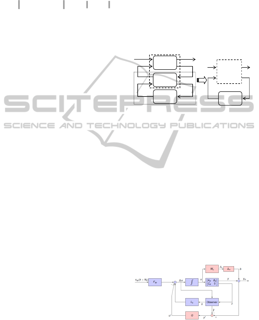
4 ROBUSTIFIED MPC
This subsection focuses on the procedure used to
enhance robustness to the Model Predictive Control
law developed in the Section 3.2. The basic idea is
to add a stable Youla-Kučera parameter (Kučera,
1974, Youla et al., 1976) to parameterize the class of
all stabilizing controllers starting from an initial
stabilizing state-feedback controller coupled with an
observer. This approach is known in the literature as
the modified controller paradigm (Boyd and Barratt,
1991, Maciejowski, 1989) and consists into
modifying the initial stabilizing controller by adding
an auxiliary input
u
and an output y
with a zero
transfer in between Fig. 2). This procedure enables
to find a controller belonging to the class of all
stabilizing controllers that will improve the
robustness of the initial control law, without
changing the initial Input/Output behaviour (i.e. the
transfer from
w to z) of the initial closed-loop in the
absence of disturbances.
Figure 2: Class of all stabilizing controllers.
The transfer
zw
T can be represented using the
LLFT (Lower Linear Fractional Transformation)
form of the initial controlled system coupled with
the Youla-Kučera parameter, denoted Q parameter,
with
0
22
zw
T
:
zwzwzw
TQTTT
zw 211211
(16)
Note that this structure is affine in the Q parameter,
allowing convex specifications in closed-loop.
The next step is to apply this strategy to the
MPC law proposed in Section 3.2. Different
scenarios can be considered depending on the choice
of the transfer
zw
T . For instance, if the aim is to
improve stability robustness under additive
unstructured uncertainties, then the following choice
has to be done
bzzw
u
TT
(Fig. 3). For robust
stability under multiplicative uncertainties, the
following transfer has to be considered
bzzw
y
TT
(Fig. 4), which is equivalent to the complementary
sensitivity function.
Figure 3: Robustification under additive unstructured
uncertainties.
y
z
u
0
K
0
21
1211
zw
zwzw
T
TT
w
w
u
u
y
y
s
K
Q
Q
z
G
ROBUSTIFIED CONTROL OF A MULTIVARIABLE ROBOT
293
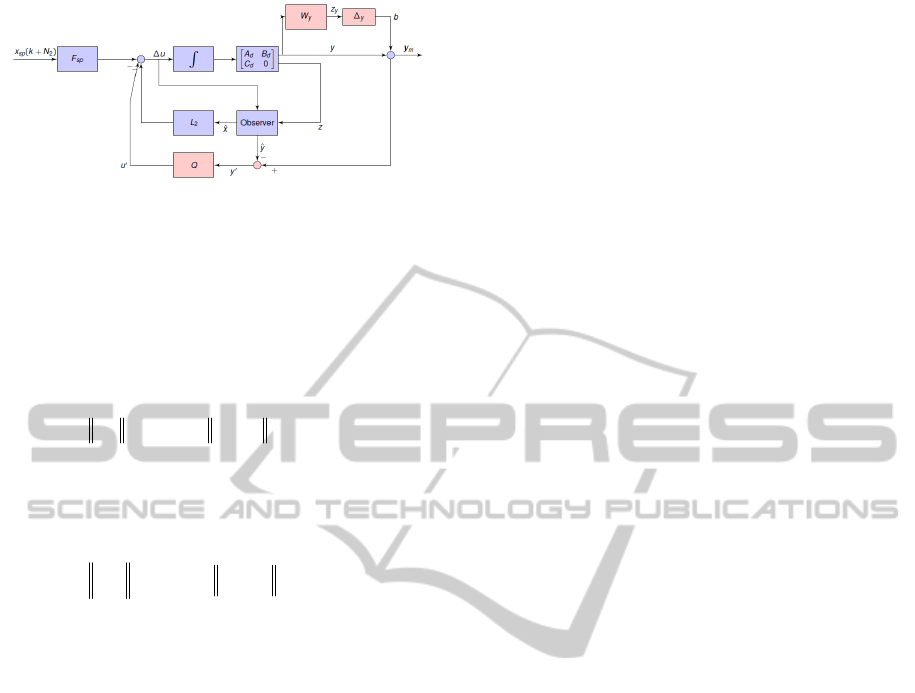
Figure 4: Robustification under multiplicative
unstructured uncertainties.
In order to improve the robustness of the initial
control the following optimization problem has to be
solved:
a. Find
HQ that improves the robust
stability under additive unstructured uncertainties
solving:
ubu
HQ
zb
HQ
TWT minmin
(17)
b.
Find
HQ that improves the robust
stability to multiplicative unstructured uncertainties
solving:
byy
HQ
bz
HQ
TWT
y
minmin
(18)
Here
u
W and
y
W denote appropriate weighting
terms chosen in order to accomplish the desired
robustness specifications in a specified frequency
range.
As the robustification procedure is identical for
both additive and multiplicative uncertainties, the
notation
zw
T will be further used for the general
case.
Since the Q parameter initially varies in the
infinite-dimensional space of stable transfers
(
H ), it is suitable to restrict the search. A sub-
optimal solution (Scherer 2000) is to consider a FIR
(Finite Impulse Response) filter. The state-space
form
QQQQ
,D,C,BA of this multivariable Q
parameter will be further used, with a known (a
priori fixed) pair
yQyQyQy
pnpnpnp
QQ
,BA
and an unknown pair
yQy
pmnpm
QQ
,DC
that will result from the optimization procedure (see
(Stoica et al., 2007) for more details). Here
Q
n
denotes the degree of the Q polynomial. The
optimization problems (17) and (18) can be
reformulated as a matrix inequality using the
following theorem.
Bounded real lemma (Boyd et al., 1994,
Scherer, 2000, Clement and Duc, 2000). A linear
discrete time invariant system with the state-space
representation
clclclcl
,D,C,BA
is stable and has a
H norm lower than
if and only if:
0
0
0
0
0
0
1
1
1
11
IγDC
DIγB
CXA
BAX
/XX
clcl
T
cl
T
cl
T
cl
T
cl
clcl
T
(19)
with “ 0 ” (“ 0 ”) denoting a strictly positive
(negative) definite matrix.
Using a change of variables and two congruence
transformations (Scherer, 2000, Clement and Duc,
2000), the expression (19 can be further transformed
into a LMI (Linear Matrix Inequality) with the
decision variables:
1
X ,
and the Q parameter
hidden in the closed-loop matrices. An exact form of
this LMI and also the entire procedure (which is
outside the aim of this paper) leading to this LMI
can be found in (Stoica et al., 2007).
Hence, depending on the considered transfer
minimisation, the resulting optimization problem is
the following:
a.
only robust stability under additive unstructured
uncertainties: minimize
subject to the Linear
Matrix Inequality
0
LMI using the state-space
representation
clclclcl
,D,C,BA
of the transfer
bzzw
u
TT
:
0
min
LMI
(20)
b.
only robust stability under multiplicative
unstructured uncertainties: minimize
subject to
the Linear Matrix Inequality
CS
LMI using the state-
space representation
clclclcl
,D,C,BA
of the transfer
bzzw
y
TT
:
CS
LMI
min
(21)
c.
robust stability under both additive and
multiplicative unstructured uncertainties: minimize a
given cost function subject to the two LMIs defined
before:
)(min
00
,
0
CSCS
LMILMI
cc
CS
(22)
ICINCO 2011 - 8th International Conference on Informatics in Control, Automation and Robotics
294
where
CS
cc ,
0
are weighting terms and
0
in
0
LMI and
CS
in
CS
LMI .
Note that this robustification procedure can be
applied to every state-feedback controller coupled
with an observer. The particular case of MPC is used
here due to its good performance and simplicity of
implementation when dealing with multivariable
systems.
5 SIMULATION RESULTS
The control strategies proposed in this paper (LQG
control, MPC and robustified MPC) are now applied
to the nonlinear model (1). The LQG and MPC
control laws are designed to achieve the same
performances and to respect the admissible motors
torques.
The LQG controller is designed in continuous-
time in accordance to an existing LQ controller
(Stoica et al., 2009) which is already implemented
on the real robot.
The linearized continuous-time model (3) used
to design the LQG control law was obtained via the
Matlab
®
function ‘linmod’. A sample time
005.0
s
T s and a zero-order hold on the inputs
discretization method were used to determine the
prediction model (9) used by MPC.
5.1 Tuning Parameters
First of all, based only on the information of the
angular position sensors from the Pivot and C-arc a
LQG controller is designed (denoted LQG
p
), using
the weighting matrices
)10,10diag(
97
1
J
R and
)4000,5000,80,50,80,20,1,1,1,1diag(
1
J
Q . The
observer weightings are chosen as
)1.0,1.0,10,10diag(
66
1
W
and
T
cc
BBV
1
,
with
5
10
.
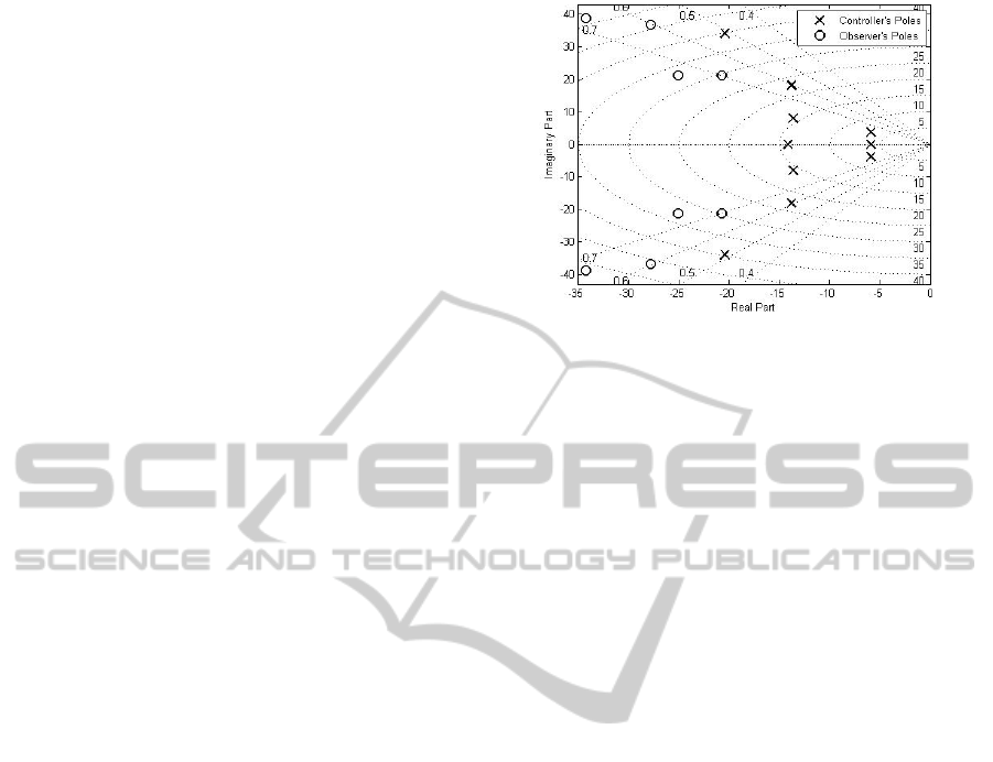
Another LQG controller (denoted LQG
a
) which
uses additional information from the accelerometers
is next developed. This increases the initial
robustness of the controller. The poles of the closed-
loop obtained with LQG
a
are presented in Fig. 5.
Secondly, the initial MPC (denoted MPC0) is
designed with the following tuning parameters:
),,,diag( ,14N,58N,8
00u21
2
JJJ
RRRN
87
0
10,10diag
J
R ,
00
,,diag
2
JJJ
QQQ
,
30,30,30,80,1,1,1,1diag
0
J
Q .
Figure 5: Closed-loop LQG
a
poles.
The MPC controller uses the information of both
angular positions and accelerations of the Pivot and
C-arc.
Thirdly, two robustified controllers are further
developed:
a.
RMPC0 that considers only robust stability
under additive unstructured uncertainties,
obtained from MPC0 with the Q parameter
which is the solution of (20);
b.
RMPC1 that takes into account robust stability
under both additive and multiplicative
unstructured uncertainties. This robustified
controller is obtained from MPC0 coupled with
the Q parameter from (22). The coefficients
50 and 1
0
CS
cc are used in the optimization
problem (22).
In both cases the degree of the Q polynomial is
chosen equal to
10
Q
n
. The weighting
u
W (Fig. 3)
on the control increment is chosen as a high-pass
filter
05.0/)95.01(
1
zW
u
and the weighting
y
W
(Fig. 4) is chosen as 1.0/)9.01(
1
zW
y
, in
order to favor the high frequency range. The total
number of scalar decision variables associated with
the LMI problem (20) is 948 and with the LMI
optimisation problem (22) is 1387.
5.2 Frequency Analysis
In the case of a multivariable system, the classical
criteria for the analysis of stability margins such as
the Nyquist criterion are no longer valid. This is the
main reason why an analysis of the maximal
singular values, which can give a meaningful
assessment of the robustness of the controlled
system, is further proposed.
In a first stage, the maximal singular values of
the transfer from
b to u obtained with the LQG
ROBUSTIFIED CONTROL OF A MULTIVARIABLE ROBOT
295
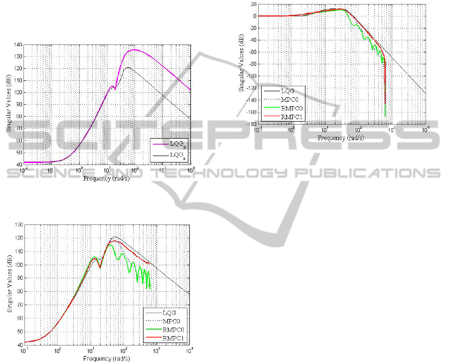
controller that uses only the motor shaft positions
(LQG
p
) and for the LQG with additional
measurements of the joints accelerations (LQG
a
) are
illustrated in Fig. 6. A significant improvement of
the controlled system behavior with the LQG
a
controller can be noticed at the high frequency
range. Thus the LQG
a
controller is kept for further
comparisons with MPC0, RMPC0 and RMPC1. For
simplicity reason the LQG
a
controller is further
denoted LQG.
Figure 6: Maximal singular values for the transfer from b
to u.
Figure 7: Maximal singular values for the transfer from b
to u.
In a second stage, a comparative analysis of the
maximal singular values from b to u is offered in
Fig. 7. The
H norm of transfer
ub
T (which is the
maximum of the maximal singular values) is
progressively decreased from LQG to MPC0 and
then to RMPC0. The MPC and the robustified MPC
controllers have better frequency responses in the
high frequency range than the LQG controller. The
robustified controller RMPC1 offers a good trade-
off in terms of
H norm between MPC0 and
RMPC0.
From the analysis of the maximal singular values
of the complementary sensitivity function depicted
in Fig. 8, the LQG controller has the largest
bandwidth leading to a better behavior in the time
domain. The
H norm of the transfer
by
T
is very
similar for all the considered controllers.
Figure 8: Maximal singular values of the complementary
sensitivity function.
5.3 Time Domain Comparison
The time domain responses are obtained using a step
set-point of magnitude
1.0
2
sp
rad for the pivot
and
15.0
3
sp
rad for the C-arc. A step
disturbance of magnitude 200Nm at time 2s on both
axes was also considered.
Figure 9 presents the outputs
m
q of the
nonlinear model of the 2 axes of the robot. All the
controllers offer good tracking, a time response
without overshoot (which is imposed by the demand
specifications) and an admissible disturbance
rejection. The time responses are very similar for all
the controllers (
s72.0
rPivot
t and s62.0
rCarc
t ).
The LQG controller offers the fastest disturbances
rejection. The disturbances rejection is slower after
robustification, which was expected due to the
frequency domain behavior. In fact the Youla-
Kučera parameter will improve the robust stability
under additive uncertainties and will slow down the
disturbances rejection. The controller RMPC1 offers
a good trade-off between the considered controllers
(see the corresponding zoom of Fig. 9).
ICINCO 2011 - 8th International Conference on Informatics in Control, Automation and Robotics
296
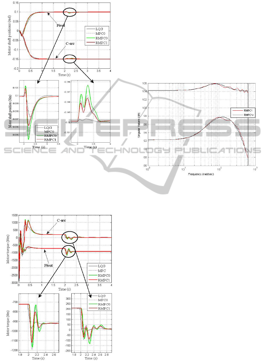
Figure 9: Output
m
q – Motor shaft positions comparison.
Figure 10 shows the control signals applied on
the nonlinear model. All the controllers offer
admissible control signals that can be implemented
on the real robot. A small oscillation (which could
come from numerical problems) can be seen on the
LQG controller.
Figure 10: Control signals – Motor torques comparison.
The robust synthesis algorithms, usually offer
large controllers. In this case the Youla-Kučera
parameter increases the dimension of the RMPC1
controller with 20 states. In order to reduce the
controller states a balanced reduction of the Youla-
Kučera parameter based on the Hankel singular
values is considered. The final controller (denoted
RMPC1r) uses a reduced Youla-Kučera parameter
that has only 4 states. Figure 11 illustrates the
singular values of the Youla-Kučera parameter
before and after the order reduction.
Figure 11: Singular values of Youla parameter before and
after order reduction.
The influence of an unstable transmission zero
(determining the behavior at the beginning of the
simulation) over the pivot axis can be easily noticed
in Fig. 9 and Fig. 10. The existence of this unstable
zero explains the choice of the prediction horizons
114N,18
u1
N .
A robust analysis of the results is also proposed.
The aim is to verify the stability of the controllers
with the nonlinear model, considering structured
uncertainties on the joint stiffness
K
and motor
inertia
m
J . Only RMPC1 and RMPC1r remain
stable for all the considered parameters variations as
synthesised in Table 1, where the following
notations have been used:
-
Case 1: KK %20
;
-
Case 2: KK %20
;
-
Case 3:
mm
JJ %20
;
-
Case 4:
mm
JJ %20
.
ROBUSTIFIED CONTROL OF A MULTIVARIABLE ROBOT
297
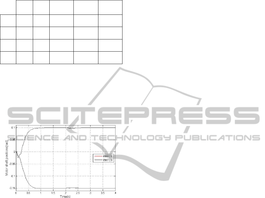
Table 1: Structured uncertainties robustness.
LQG MPC RMPC0 RMPC1
RMPC1r
Case 1
Case 2
Case 3
Case 4
Figure 12 illustrates the case where an
uncertainty of
%20 is considered on the motors
inertia:
mm
JJ %20 . Despite this uncertainty and
the nonlinearities of the system, the robustified
controller RMPC1 still stabilises the system.
Moreover, it can be observed that this property is
conserved even after the order reduction.
Figure 12: Output
m
q . Nonlinear model with
uncertainties of
mm
JJ %20
.
6 CONCLUSIONS
This paper proposes a comparison between
advanced control techniques for the control of the
angular position of a two axes model of a
cardiovascular robot, which is a strongly nonlinear
multivariable system. In order to improve the
controllers’ robustness, several layers of
robustification are further considered.
A linear quadratic controller (LQG) and a Model
Predictiv Control (MPC) law are first designed to
achieve similar level of performance for the time-
domain response. In a first step, additional
measurements of the joints accelerations are used in
order to increase the initial level of robustness of the
two controllers. Robust stability under unstructured
uncertainties is explicitly considered in the synthesis
of the robustified MPC controllers, while, for the
LQG controller, the robust stability under
unstructured uncertainties is verified a posteriori.
Simulation results show a trade-off between robust
stability and disturbances rejection.
The robustness towards the variation of some
parameters (i.e. structured uncertainties) is verified a
posteriori for all the considered controllers. An
interesting perspective is to take into account these
structured uncertainties during the synthesis of the
robustified MPC. A possibility is to consider a
polytopic uncertain domain around the nominal
model as in (Stoica et al., 2009) and to guarantee the
stability over the specified uncertain polytopic
domain solving a BMI (Biliniar Matrix Inequality)
optimisation problem.
REFERENCES
Al Assad, O., Godoy, E., Croulard, V., 2008. Macroscopic
drive chain efficiency modeling using state machines.
17th IFAC World Congress, Seoul, pp. 2294-2299.
Al Assad, O., Godoy, E., Croulard, V., 2007.
Irreversibility modeling applied to the control of
complex robotic drive chains. 4th ICINCO, Angers,
pp. 217-222.
Book, W. J., 1989. Modelling, design, and control of
flexible manipulators arms: status and trends. NASA
Conference on Space Telerobotics, vol. 3, pp. 11-24.
Boyd, S., Barratt, C., 1991. Linear controller design.
Limits of performance, Prentice Hall.
Boyd, S., Ghaoui, L. El., Feron, E., Balakrishnan, V.,
1994. Linear matrix inequalities in system and control
theory, SIAM Publications, Philadelphia.
Camacho, E. F., Bordons, C., 2004. Model predictive
control, Springer-Verlag. London, 2
nd
edition.
Clement, B., Duc, G., 2000. A multiobjective control via
Youla parameterization and LMI optimization:
application to a flexible arm, IFAC Symposium on
Robust Control and Design, Prague.
Doyle, J. C., Stein, G., 1979. Robustness with observers.
In IEEE Trans. Automatic Control, vol. AC 24, pp.
607-611.
Halalchi, H., Bara, G. I., Laroche E., 2010. LPV controller
design for robot manipulators based on augmented
LMI conditions with structural constraints, IFAC
Symposium on System, Structure and Control, Ancona,
Italy.
Hedjar R., Toumi, R., Boucher, P., Dumur, D., 2002.
Feedback nonlinear predictive control of rigid link
robot manipulators, IEEE ACC, Anchorage, AK,
USA, pp. 3594-3599.
Kučera, V., 1974. Closed loop stability of discrete linear
single variable systems, Kybernetika, vol. 10(2),
pp. 146-171.
Maalouf, A.I., 2006. Improving the robustness of a
parallel robot using Predictive Functional Control
ICINCO 2011 - 8th International Conference on Informatics in Control, Automation and Robotics
298

(PFC) tools, 45th IEEE CDC, San Diego, CA, USA
pp. 6468-6473.
Maciejowski, J. M., 2001. Predictive control with
constrains, Prentice Hall.
Maciejowski, J. M., 1989. Multivariable feedback design,
Addison-Wesley Publishing Company, Wokingham.
Merabet, A, Gu, J., 2009. Generalized predictive control
for single-link flexible joint robot, International
Journal on Sciences and Techniques of Automatic
Control, vol. 3, no. 1, pp. 890-899.
Moreno-Valenzuela, J., Santibáñez, V., Campa, R., 2008.
On output feedback tracking control of robot
manipulators with bounded torque input, International
Journal of Control, Automation, and Systems, vol. 6,
no. 1, pp. 76-85.
Sciavicco, L., Siciliano, B., 1996. Modelling and control
of robot. McGraw-Hill Company, Inc., New York.
Scherer, C. W., 2000. An efficient solution to multi-
objective control problem with LMI objectives.
Systems and Control Letters, 40, pp 43-57.
Spong, M. W., Hutchinson, S., Vidyasagar, M., 2005.
Robot modeling and control, John Wiley Sons Inc.,
2005.
Spong, M. W., 1992. On the robust control of robot
manipulators, IEEE Transactions on Automatic
Control, vol. 37, pp. 1782-1786.
Stoica, C., Rodríguez-Ayerbe, P., Dumur, D. 2007.
Improved robustness of multivariable Model
Predictive Control under model uncertainties, 4th
ICINCO, Angers, France, pp. 283-288.
Stoica, C., Al Assad, O., Rodriguez-Ayerbe, P., Godoy, E.
Dumur, D., 2009. Control of a flexible arm by means
of robustified MPC, European Control Conference,
Budapest, Hungary, pp. 2229-2234.
Tomei, P., 1994. Tracking control of flexible joint robots
with uncertain parameters and disturbances, IEEE
Transactions on Automatic Control, vol. 39, no. 5, pp.
1067-1072.
Youla, D. C., Jabr, H. A., Bongiorno Jr., J.J., 1976.
Modern Wiener-Hopf design of optimal controllers –
part II : the multivariable case, IEEE Transactions on
Automatic Control, vol. 21(3), pp. 319-338.
ROBUSTIFIED CONTROL OF A MULTIVARIABLE ROBOT
299
