
VISUAL OUTDOOR PATH PLANNER FOR ORANGE GROVES
BASED ON ENSEMBLES OF NEURAL NETWORKS
Joaqu´ın Torres-Sospedra and Patricio Nebot
Departamento de Ingenier´ıa y Ciencia de los Computadores, Universitat Jaume I
Avda. Sos Baynat S/N, E-12071, Castell´on, Spain
Keywords:
Outdoor mobile robotics, Agricultural environments, Visual path planner, Ensembles of neural networks.
Abstract:
One of the most important system to deploy for a robot navigating in an outdoor scenario, as can be an orange
grove, is the navigation system. In this paper, a path planner in orange groves for an autonomous robotic
system is presented. This path planner is based on a previous classification of the image that the robot gets
from its visual sensory system. One of the most important technique used to generate accurate classifiers
is based on training an ensemble of neural networks. Here, a simple ensemble of neural networks is used to
classify images from an orange grove using wavelets features. With the classification image obtained, the most
important lines of the land are extracted with the Hough transform. The final path line is determined with these
lines. The purpose of this paper is to determine if the ensemble approach can be useful in the procedure to
design an accurate path planner for outdoor autonomous robots in orange groves. The published results show
that ensembles can be considered for this type of applications.
1 INTRODUCTION
Ensembles of neural networks are commonly applied
to solve classification problems. It has been demon-
strated that an ensemble with uncorrelated networks
provides better generalization than a single network
(Raviv and Intratorr, 1996; Tumer and Ghosh, 1996).
The main goal of this research is to provide an au-
tonomous path planner to a robot that navigates into
an orange grove. To perform this task, a neural net-
work based system will be applied to determine the
areas as Sky, Land, Orange trunks and Orange Crown.
With this information, it is possible to determine the
boundaries of the land with the other classes and then
calculate the path the robot should follow.
In this paper, a basic ensemble of neural networks
is introduced in order to classify the images from an
orange grove. To perform the classification task, some
wavelet features from the image will be processed by
the ensemble according to (Sung et al., 2010).Once
the classification is done, the information provided by
the ensemble will be used to obtain the boundaries of
the land with the orange trunks and the other classes.
To calculate the border lines, the Hough transform
is used. With these lines, the application calculates
the desired path line which the robot should follow.
This path line along with other information obtained
with GPS and satellite maps will be send to the navi-
gation module to establish the final robot route.
The process of designing an ensemble of neural
networks consists of two main steps. In the first step,
the development of the ensemble, the networks are
trained according to the specifications of the ensem-
ble method. The second step, the determination of the
suitable combiner, focuses in selecting the most accu-
rate combiner for the generated ensemble.
As it has been previously mentioned, the classi-
fiers of an ensemble are more useful when they make
independent errors. Furthermore, some authors de-
fend that the error of the ensemble decreases as diver-
sity increases (Tumer and Ghosh, 1996). There are
some sources or ways to create different neural net-
works with a increase in the diversity of the system.
The rest of paper is organized as follows. In Sec-
tion 2, the description of the classification system is
introduced. In Section 3, the whole process to detect
the desired path is described. The experimental setup
and some preliminary results are shown Section 4.
223
Torres-Sospedra J. and Nebot P..
VISUAL OUTDOOR PATH PLANNER FOR ORANGE GROVES BASED ON ENSEMBLES OF NEURAL NETWORKS.
DOI: 10.5220/0003537602230228
In Proceedings of the 8th International Conference on Informatics in Control, Automation and Robotics (ICINCO-2011), pages 223-228
ISBN: 978-989-8425-75-1
Copyright
c
2011 SCITEPRESS (Science and Technology Publications, Lda.)

2 CLASSIFICATION OF THE
IMAGES
2.1 Multilayer Feedforward Network
Firstly, the network architecture used in the experi-
ments performed in this paper is the Multilayer Feed-
forward Network, henceforth called MF network.
This kind of networks consists of three layers of
computational units. The neurons of the first layer
apply the identity function whereas the neurons of the
second and third layers apply the sigmoid function.
This network can approximate any function with a
specified precision (Bishop, 1995; Kuncheva, 2004).
In the case of the application described in this pa-
per, the networks have been trained for a few itera-
tions. In each iteration, the weights of the networks
have been adapted with the Backpropagation algo-
rithm by using all the patterns from the training set,
T. At the end of the iteration the Mean Square Error,
MSE, has been calculated by classifying all the pat-
terns from the the Validation set, V. When the learn-
ing process has finished, the weights of the iteration
with lowest MSE of the validation set are assigned to
the final network. The learning process is described
in Algorithm 1.
Algorithm 1: MF Network Training{T ,V}.
Set initial weights randomly
for e = 1 to epochs do
for i = 1 to N
patterns
do
Select pattern x
i
from T
Adjust the trainable parameters
end for
Calculate MSE over validation set V
Save epoch weights and calculated MSE
end for
Select epoch with lowest error
To perform the experiments, the original dataset
has been divided into three different subsets. The first
set is the training set, T, which is used to adapt the
weights of the networks (64% of total patterns). The
second set is validation set, V, which is used to se-
lect the final network configuration (16% of total pat-
terns). Finally, the last set is the test set, TS, which
is applied to obtain the accuracy of the network (20%
of total patterns). The original learning set, L, refers
to the training and validation sets, the sets which are
involved on the learning procedure.
2.2 The Ensemble of Neural Networks
The process of designing an ensemble of neural net-
works consists of two main steps. In the first step,
the development of the ensemble, the networks are
trained according to the specifications of the ensem-
ble method. The second step, the determination of the
suitable combiner, focuses in selecting the most accu-
rate combiner for the generated ensemble.
As has been previously described, the learning
process of an artificial neural network is based on
minimizing a target function. A simple procedure to
increase the diversity of the classifier consists in using
several neural networks with different initial values of
the trainable parameters. Once the initial configura-
tion is randomly set, the networks can be trained as a
single network. With this ensemble method, known
as Simple Ensemble, the networks converge into dif-
ferent final configurations(Dietterich, 2000) therefore
diversity and performance of the system can increase.
Its description is shown in Algorithm 2.
Algorithm 2: Simple Ensemble {T ,V N
networks
}.
Generate N
networks
different seed values: seed
i
for i = 1 to N
networks
do
Random Generator Seed = seed
i
Original Network Training {T , V}
end for
Save Ensemble Configuration
Finally, the output of the networks are averaged
in order to get the final output of the whole system.
This way to combine an ensemble is known as Output
average or Ensemble Averaging.
2.3 Codification of the Problem
To perform the classification task, some wavelet fea-
tures from the image will be processed by the en-
semble according to (Sung et al., 2010). To deter-
mine the classification, the image is divided into NxM
blocks, instead of working directly with the pixels.
Concretely, the two-level Daubechies wavelet trans-
form - ‘Daub2’ is applied to each HSI channel of the
image. Then, the features Mean and Energy of the
wavelet sub-bands are calculated for each HSI chan-
nel and image block. With this procedure, 14 features
can be extracted for each HSI channel. Some of them
can not be used due to noise.
In the system, a pattern is represented by a 26-
dimensional vector (8 wavelet features for each HSI
channel and the 2 spatial coordinates) which is pre-
sented to the network in order to classify the origi-
nal image block by block. This vector is successfully
used to classify images of orange groves. However,
since the structure of orange groves is very delimited,
probably the number of features could be reduced and
the computational cost of the classification could be
lower, but this aspect has not been tested yet.
ICINCO 2011 - 8th International Conference on Informatics in Control, Automation and Robotics
224
3 PATH PLANNER FOR
NAVIGATION IN ORANGE
GROVES
The classification task has been introduced in the sec-
ond section of the paper. However, the classification
of each block of the image must be processed in or-
der to obtain the path the robot should follow. The
process to obtain the path from the classification is
described in this section.
3.1 Generating the Output Image
First of all, the output image must be generated. This
artificial image represents the class of each block of
the original image.
Each block of the image has been processed by
an ensemble of neural networks to calculate the cor-
responding class as described in the previous section.
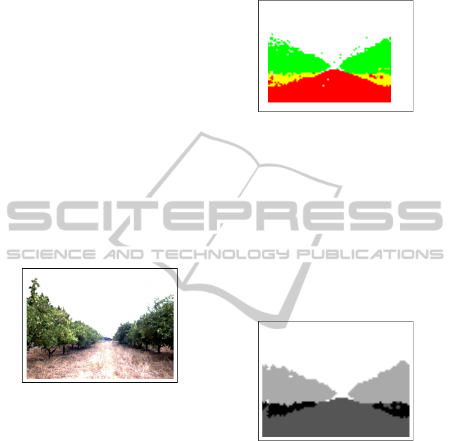
Figure 1 shows a original image taken at an orange
grove, whereas its classification is represented in Fig-
ures 2 and 2.
Figure 1: Photo taken atan orange grove placed in Vila-real.
In this photography, there are some orange trees
at the left and right sides of the image. The land is
located at the bottom of the image and the sky is at
the top. This basic structure which can be seen in
the original image tends to be similar in most of the
orange groves. To process the original image an en-
semble of neural networks has been trained with the
Simple Ensemble method. Figure 2 shows how this
ensemble has classified each block of the image.
In the classification image the colors are organized
as follows: red refers to Land, white is Sky, green is
Orange crown and yellow refers to the area of Orange
trunk. It can be seen how the classification is accurate
and the important areas are correctly classified. It is
possible to see the basic structure of the orange grove
in the classification image. Although this classifica-
tion image is representative for humans, it is neces-
sary to generate a classification picture in gray scale
in order to process it and obtain the path lines.
Figure 2: Classification of the example image - Color.
3.2 Filtering the Output Image
Although the classification obtained with the ensem-
ble is accurate, most of the errors are located in the
boundaries between objects (classes). For this reason,
some image filters are necessary to apply in order to
reduce the errors and obtain precisely the path.
First of all, all the isolated blocks are removed.
The class associated to a block is reassigned if it is
not surrounded by another block of the same class.
Then an erode/dilate filter is used to remove small
wrong areas. Moreover, the filter to eliminate all the
isolated blocks can be applied again. The classifica-
tion image after filtering is shown in Figure 3.
Figure 3: Classification image after filtering.
The applied filters have been selected because
they are fast, an important feature in our real time sys-
tem, and the results are good enough. After these pro-
cedures, the image can processed to extract the path.
3.3 Detecting Borders and Lines
With the filtered classification image and the structure
of the orange grove, it is possible to determine the
path by detecting the main lines between the land and
each orange tree row. The Hough transform has been
applied to detect these lines of the image.
In this application, an edge detector is required as
a pre-processing stage to obtain the blocks that are on
VISUAL OUTDOOR PATH PLANNER FOR ORANGE GROVES BASED ON ENSEMBLES OF NEURAL
NETWORKS
225
the desired lines in the image space because the lines
which must be detected are the borders of the filtered
classification image. After some review in border de-
tection algorithms, ‘canny’ algorithm was chosen.
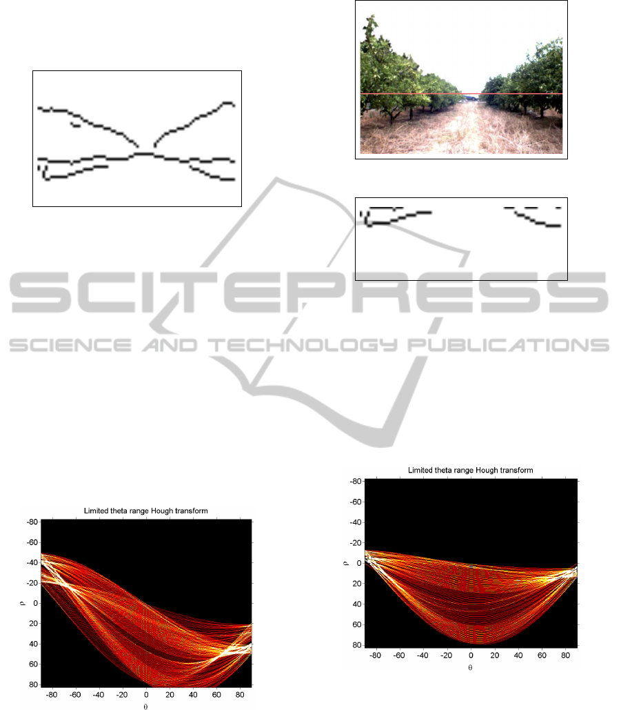
Figure 4: Borders between classes.
Figure 4 shows the image obtained after applying
the ‘canny’ algorithm. At first sight, the five repre-
sentative lines which represents the borders between
classes can be seen. From these five lines, only three
of them have to be extracted. The horizontal line and
the two lines located at the bottom part of the image.
Although the other two lines are also important they
are not used at this stage of the system.
To extract the three lines of interest for the appli-
cation, Hough transform is applied and a matrix with
all the lines possibles is generated. The lines are rep-
resented with Hesse equation, so they depend on an
angle θ and a distance ρ. Figure 5 shows the Hough
transform for the example. The lightest parts repre-
sent the most representative lines, the lines with high-
est number of votes.
Figure 5: Hough transform of the filtered classification.
First of all, the most representative horizontal line
is extracted. For the angle which represents the hori-
zontal lines, θ equal to −90, the distance ρ with high-
est vote is chosen to generate the line. Figure 6 shows
the original image along with the detected horizontal
line. This line has been calculated because the path
line must be located under it.
Figure 6: Example image with the main horizontal line.
Figure 7: Borders of the reduced classification.
Then the Hough transform is applied to the bottom
part of the image (shown in Figure 7) to detect the
borders between land and orange trunks. The bottom
part of the image corresponds to the blocks located
below the horizontal line detected in the previousstep.
Figure 8 shows the second transform in which the
borders between land and orange trunks are detected
with simple lines.
Figure 8: Hough transform - reduced classification.
In this second representation, it is easy to see that
due to its simplicity, the detection of the two lines can
be faster than applying it to the entire image. The left
border is represented with a positive angle whereas
a negative angle represents the right border. These
two lines are plot over the original image is shown in
Figure 9.
ICINCO 2011 - 8th International Conference on Informatics in Control, Automation and Robotics
226
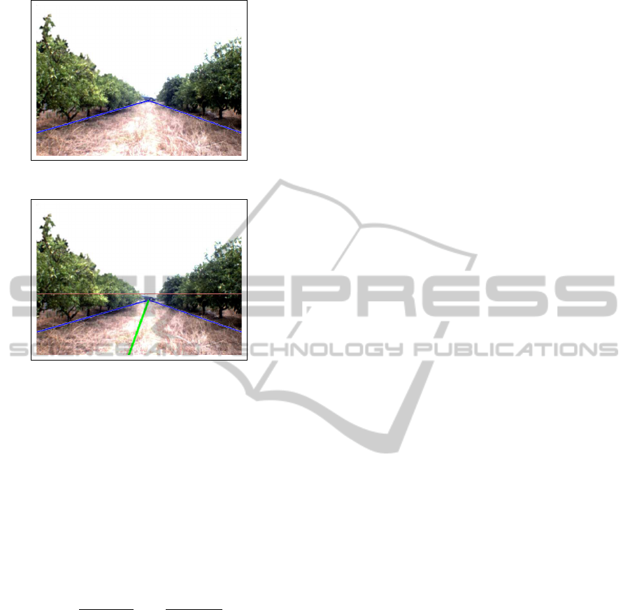
Figure 9: Example image with the representative borders.
Figure 10: Example image with the representative lines
(borders and path).
3.4 Establishing the Path
Once the two representative lines are extracted, the
path can be calculated with them. Concretely, the
path corresponds to the line between them. Figure
10 shows the orange grove where the horizontal main
line (red), the borders between land and trunks (blue)
and the path line (green) are plot over it.
This path is represented with two parameters of
the Hesse equation, ρ
path
and θ
path
.
y =
ρ
path
sin(θ
path
)
− x·
cos(θ
path
)
sin(θ
path
)
(1)
With these two parameters, the robot can know its
displacement and inclination with respect to the cen-
ter of the path. They will be used along with GPS
information and other maps to calculate the distance
to intermediate points and correct the path trajectory
to navigate into the orange grove.
4 EXPERIMENTAL SETUP AND
RESULTS
4.1 Experiments
In the application described, an ensemble of 9 MF
networks has been trained using a few test images.
This size, nine networks in the ensemble, has
been chosen because it reports good results according
to (Fernndez-Redondo et al., 2004; Torres-Sospedra
et al., 2005) and the computational costs do not shoot
up.
4.1.1 Network Parameters
The MF networks used in the experiments have the
following structure: 26 input parameters, 10 hidden
units and 4 output classes. Each output unit is related
to the probability associated to an output class. The
output vectors provided by the nine networks are av-
eraged. The predicted class for an image block corre-
sponds to the output unit of the averaged vector with
highest value.
The Backpropagation parameters used to train the
networks are the following ones: 1000 iterations, 0.2
as adaptation step and 0.05 as momentum rate.
All these parameters, have been set after an ex-
haustive trial-and-error procedure in which some con-
figurations have been tested. The configuration which
reports the best performance on a common validation
set has been chosen for the experiments.
4.1.2 Block Image Parameters
As explained in section 2.3, the classification task is
not applied directly over the pixels. Instead, the image
is divided into N×M blocks of pixels, being N and M
any number.
To perform the experiments presented in this pa-
per, and after some empirical tests, the block size is
set to 8×8 pixels.
All the captures shown in this paper were taken
with a VGA FOculus camera.
4.2 Results
An ensemble of neural networks has been used to cal-
culate the path in some images. In Figure 11, four
different images of orange groves used to test the ap-
plication are shown.
In these images, the path and the other important
lines calculated by the application are also shown. It
is important to remark that the original images of the
orange groves were taken with different light condi-
tions and different positions in the orange rows.
As it can be seen, the path tends to be accurate
enough for the navigation. However, it would be rec-
ommendable to optimize the classification system to
improve the performance and accuracy of the path
planner.
VISUAL OUTDOOR PATH PLANNER FOR ORANGE GROVES BASED ON ENSEMBLES OF NEURAL
NETWORKS
227
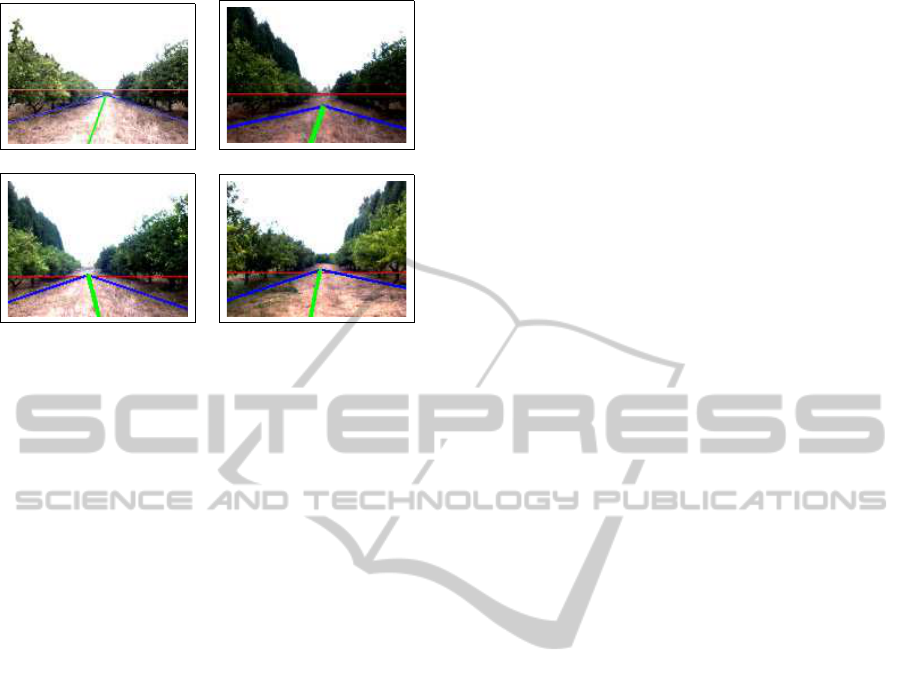
Figure 11: Some results and their representative lines.
5 CONCLUSIONS
In this paper, a system used to successfully classify
the different elements of an orange grove is presented.
This classification system is based on the classifica-
tion of a orange grove image with features extracted
from the wavelets of each channel of the HSI color
space. Moreover, in the work presented in this pa-
per, an ensemble of simple neural networks has been
used instead of a classic classifier based on a lonely
network with two hidden layers.
With the use of the ensemble of neural networks,
the results of the classification are very promising.
In fact, based on the prediction of the ensemble, it
has been presented a procedure to calculate the path
that the robot should follow to navigate by the ore-
nage grove. Moreover, in the future, this classifica-
tion could be used to perform other tasks, such as de-
termine zones where to apply a certain maintenance
orange grove work.
Further work will be focused on generating better
classifiers with the new data that is being collected.
In the paper has been demonstrated that Simple En-
semble is accurate enough to perform our classifica-
tion tasks. However, there are other ensemble meth-
ods which have been demonstrated that are better.
These other advanced methods, such as those based
on Boosting (Oza, 2003) and Cross-Validation Com-
mittee (Verikas et al., 1999), could be used in further
experiments to optimize the classification task.
ACKNOWLEDGEMENTS
This paper describes research carried out at the
Robotic Intelligence Laboratory of Universitat
Jaume-I. Support is provided in part by the General-
itat Valenciana under project GV/2010/087, and by
the Fundaci´o Caixa Castell´o - Bancaixa under project
P1-1A2008-12.
REFERENCES
Bishop, C. M. (1995). Neural Networks for Pattern Recog-
nition. Oxford University Press, Inc., New York, NY,
USA.
Dietterich, T. G. (2000). Ensemble methods in machine
learning. In Kittler, J., editor, Multiple Classifier Sys-
tems., number 1857 in LNCS, pages 1–15.
Fernndez-Redondo, M., Hernndez-Espinosa, C., and
Torres-Sospedra, J. (2004). Multilayer feedforward
ensembles for classification problems. In Pal, N. R.,
Kasabov, N., Mudi, R. K., Pal, S., and Parui, S. K.,
editors, Neural Information Processing, 11th Inter-
national Conference, ICONIP 2004, Calcutta, India,
November 22-25, 2004, Proceedings, volume 3316 of
Lecture Notes in Computer Science, pages 744–749.
Springer. ISBN: 3-540-23931-6.
Kuncheva, L. I. (2004). Combining Pattern Classifiers:
Methods and Algorithms. Wiley-Interscience.
Oza, N. C. (2003). Boosting with averaged weight vectors.
In Multiple Classifier Systems, volume 2709 of LNCS,
pages 15–24. Springer.
Raviv, Y. and Intratorr, N. (1996). Bootstrapping with noise:
An effective regularization technique. Connection Sci-
ence, Special issue on Combining Estimators, 8:356–
372.
Sung, G.-Y., Kwak, D.-M., and Lyou, J. (2010). Neu-
ral network based terrain classification using wavelet
features. Journal of Intelligent and Robotic Systems,
59(3-4):269–281.
Torres-Sospedra, J., Hernndez-Espinosa, C., and Fernndez-
Redondo, M. (2005). New results on ensembles of
multilayer feedforward. InArtificial Neural Networks:
Formal Models and Their Applications., volume 3697
of Lecture Notes in Computer Science, pages 139–
144. Springer.
Tumer, K. and Ghosh, J. (1996). Error correlation and error
reduction in ensemble classifiers. Connection Science,
8(3-4):385–403.
Verikas, A., Lipnickas, A., Malmqvist, K., Bacauskiene,
M., and Gelzinis, A. (1999). Soft combination of neu-
ral classifiers: A comparative study. Pattern Recogni-
tion Letters, 20(4):429–444.
ICINCO 2011 - 8th International Conference on Informatics in Control, Automation and Robotics
228
