MODELING AND SIMULATING A NARROW TILTING CAR
Salim Maakaroun, Wisama Khalil, Maxime Gautier and Philippe Chevrel
Institut de Recherche en Communication et Cybernétique de Nantes, 1 rue de la Noe, Nantes 44321, France
Keywords: Intelligent Transportation Systems, Modelling, Simulator, Robotics, Tilting car.
Abstract: The use of an electrical narrow tilting car instead of a large gasoline car should significantly decrease traffic
congestion, pollution and parking problem. The aim of this paper is to give an approach to develop a
dynamic model for narrow cars. This model can be used to simulate their behaviours and evaluate tilt
control systems. The approach is based on considering the vehicle as a multi-body poly-articulated system
and the modelling is carried out using the robotics formalism based on the modified Denavit-Hartenberg
geometric description.
1 INTRODUCTION
The idea behind narrow tilting car research is to
develop a vehicle used in urban transportation
having the advantages of motorcycle and passenger
car. This will reduce the size of the vehicle such that
it can be operated on reduced size lanes thereby
increasing the effective capacity of highways. In
order to maintain its stability, the vehicle should tilt
while cornering, to compensate the effect of lateral
acceleration and remain in its trajectory. Moreover
the use of electric motors with a group of batteries is
the most earth friendly technology.
In the literature, many works have been
published on the topic of tilting narrow vehicle.
Karnopp and Fang (Karnopp, 1992) were the first to
suggest a leaning into the turn similar like
motorcyclist’s one. Karnopp, Hibbard and So
(Hibbard, 1992. So, 1997) studied the tilt angle
required and the dynamics of such a vehicle. But
few people talked about the global dynamic model
of a four wheel tilting car. Rajamani, Gohl and
Alexander (Gohl, 2006) developed a dynamic model
of a three wheel vehicle which has four degrees of
freedom including lateral and tilt dynamics. All
these models don’t take into account the dynamics
of the suspensions, the vertical dynamic and the
study was on a simplified model called bicycle
model. Therefore to model a complex system in 3D
motion, many methods can be used. Kiencke
described his model with 4 individual co-ordinate
systems (Kiencke, 2000) while Rajamani with 6 co-
ordinate system (Rajamani, 2006). We claim that it
is preferable to proceed in a systematic method of
geometrical description, based on the modified
Denavit-Hartenberg parameterization (Khalil, 1986).
The last was applied on a two wheeled vehicle
model with suspensions (Maakaroun, 2011). This
description allows to automatically calculate the
symbolic expression of the geometric, kinematic and
dynamic models by using a symbolic software
package SYMORO+ (Symbolic Modelling of
Robots) (Khalil, 1997). Moreover, the dynamical
model can be calculated numerically using
programming software as Matlab, C++. This
formulation leads to a minimum set of equations
where the constraint equations for the mechanical
system are automatically eliminated.
This paper concentrates on developing a global
dynamic model for a narrow tilting car “Lumeneo
Smera “ (Lumeneo, 2003) by applying methods used
in robotics. Since the structure of the Smera is
complex and contains loops, this approach can
elaborate systematically the symbolic equations of
motion and makes the implementation of the
dynamic model very easy. This method is described
and applied on the car in section 2. Then Kinematics
and dynamics models are given in section 3 and 4.
Finally, simulation results are illustrated and
commented and conclusions are done.
2 GEOMETRIC DESCRIPTION
OF THE CAR
2.1 Robotic Representation of a
Multi-body System
The car is considered as a mobile tree-structured
229
Maakaroun S., Khalil W., Gautier M. and Chevrel P..
MODELING AND SIMULATING A NARROW TILTING CAR.
DOI: 10.5220/0003538102290235
In Proceedings of the 8th International Conference on Informatics in Control, Automation and Robotics (ICINCO-2011), pages 229-235
ISBN: 978-989-8425-75-1
Copyright
c
 2011 SCITEPRESS (Science and Technology Publications, Lda.)

multi-body system composed of n bodies (links)
where the chassis is the mobile base and the wheels
are the terminal links.
The links are numbered
consecutively from the base to the terminal links.
Each body C
j
is connected to its antecedent C
i
(i=a(j)) with a joint that represents an elastic or rigid
translational or rotational degree of freedom. The
symbol
a(j) denotes the link antecedent to link j, and
consequently a(j) < j .A body can be virtual or real;
the virtual bodies are introduced to describe joints
with multiple degrees of freedom like ball joint or
intermediate fixed frames. The frame R
i
(O
i
, x
i
, y
i,
z
i
)
which is attached to the body C
i
is defined as
following:
The z
i
axis is along the axis of joint i, the u
j
axis
is defined as the common normal between z
i
and z
j
.
The x
i
axis is along the common normal between z
i
and one of the succeeding z axis, where link i is the
antecedent of link j and the origin O
i
is the
intersection of z
i
and x
i
.
The homogeneous transformation matrix
i
T
j
between
two consecutive frames R
i
and R
j
is expressed as a
function of the following six parameters (Figure 1):
• γ
j
: angle between x
i
and u
j
about z
i
• b
j
: distance between x
i
and u
j
along z
i
• α
j
: angle between z
i
and z
j
about u
j
•d
j
: distance between z
i
and z
j
along u
j
• θ
j
: angle between u
j
and x
j
about z
j
• r
j
: distance between u
j
and x
j
along z
j
z
j
z
i
z
k
z
i
u
j
x
j
d
j b
j
O
i
C
i
C
j
C
k
x
i
=u
k
α
j
r
j
θ
j
α
k
γ
j
Figure 1: Geometric parameters.
The generalized coordinate of joint j is denoted by
q
j
, it is equal to r
j
if j is translational and θ
j
if j is
rotational. In (Figure 1), since x
i
is taken along u
k
,
the parameters γ
k
and b
k
are equal to zero. We define
the parameter σ
j
= 1 if joint j is translational and σ
j
=
0 if joint j is rotational. If there is no degree of
freedom between two frames that are fixed with
respect to each other, we take σ
j
=2. In this case, the
time derivative of q
j
is zero.
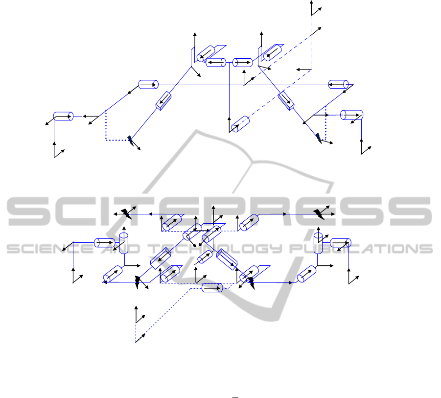
2.1 Application for the Tilting Car
The model of the Smera (Figure 2): is composed of
19 real bodies (Lumeneo, 2003) connected by 24
joints. Thus it contains 6 closed Kinematic loops:
- C
1
is the chassis
- C
2
and C
13
are two mechanical parts called “lyre”
which have a rotational movement around the
longitudinal axis of the chassis. C
2
is actuated by
an electrical motor which controls the roll of the
vehicle.
- C
5
and C
8
are the rear driving wheels.
- C
3
, C
6
and C
14
, C
15
are respectively the rear and
the front suspensions of the vehicle.
- C
4
and C
7
are the rear arms that connect the
chassis to the rear wheels.
- C
11
and C
18
are the front steering wheels.
- C
9
, C
10
and C
12
and the chassis constitute a
parallelogram which carries the hub of the left
front wheel.
- C
16
, C
17
and C
19
constitute with the chassis a
parallelogram which carries the hub of the right
front wheel;
The Kinematic closed loops are defined as follows:
- LP1 is composed of C
1
, C
2
, C
3
and C
4
- LP2 is composed of C
1
, C
2
, C
6
and C
7
- LP3 is the left parallelogram; it is composed of
C
1
, C
9
, C
10
and C
12
- LP4 is composed of C
1
, C
9
, C
13
and C
14
- LP5 is the right parallelogram composed by C
1
,
C
16
, C
17
and C
19
- LP6 is composed of C
1
, C
13
, C
15
and C
16
Let R
f
be a fixed reference frame attached to the
ground. In robots manipulator, C
0
is fixed with
respect to R
f
. In case of mobile system C
0
is taken
fixed with the chassis frame.
So according to MDH description and
SYMORO+, the structure is defined as a robot with
a mobile base by considering C
1
attached to C
0
via a
blocked joint.
The inertial parameters of this base are
those of C
1
and the speed and the acceleration are
then the ones of the chassis described in his own
frame. The chassis motion is described with Euler
coordinates (Cartesian) while all the other links are
described with the generalized Lagrangien
coordinates (joints). The body C
1
with a location ζ
(i.e. position & orientation) gives the system posture
in the frame R
f
. The movement of the chassis in this
mixed Euler-Lagrangien model is given by:
⎥
⎥
⎥
⎥
⎦
⎤
⎢
⎢
⎢
⎢
⎣
⎡
=
⎥
⎥
⎥
⎥
⎦
⎤
⎢
⎢
⎢
⎢
⎣
⎡
=
⎥
⎥
⎥
⎥
⎦
⎤
⎢
⎢
⎢
⎢
⎣
⎡
=
1
1
1
1
1
1
1
1
1
1
1
1
1
1
1
1
1
1
1
1
1
1
1
1
,,
z
y
x
z
y
x
z
y
x
V
V
V
V
ω
ω
ω
ω
ω
ω
ω
ω








It is to be noted that:
1
1
1
1
1
1
1
1
VV
dt
d
V ∧+= ω

ICINCO 2011 - 8th International Conference on Informatics in Control, Automation and Robotics
230

Where
1
V
1
= [
1
V
x1
1
V
y1
1
V
z1
]
T
are respectively the
longitudinal, lateral and vertical translational speed
of the chassis.
C
19
C
18
C
17
C
16
C
7
C
8
C
6
C
3
C
2
C
4
C
5
C
13
C
10
C
11
C
9
C
12
C
14
C
15
C
1
Figure 2: Multi-body description of the Smera.
All the joints which connect the various bodies
are revolute joints except the joints on both sides of
the rear suspensions and the joints below the front
hubs are respectively spherical and cardan joints.
The suspensions are represented by prismatic
flexible joints.
The rear Lyre is motorized, and all the joints can
be calculated in terms of this actuated joint, by
resolving the geometric equations of each loop. The
resolution of these equations was validated
experimentally (Maakaroun, 2010).
The modelling of a complex structure which
contains multiple loops is carried out by opening
each loop in order to obtain, an equivalent tree
structure system. The opened joints are chosen
among the non-motorized (passive) joints.
Loops LP1, LP2, LP3, LP4, LP5 and LP6 are
opened as shown in figure 3.
According to this description, the vehicle motion is
completely described by the vector q of the 36
generalized coordinates:
[]
T
pa
qqq =
;
[
]
T
aa
q ξξ =
;
pp
q ξ =
ξ[1x6] is the posture of the chassis ( position &
orientation)
[]
'17'108518111514632
qqqqqqqrrrq
a
=
ξ
ξ
a
is the vector of the actuated and independent
joints.
[]
21 ppp
ξξξ =
[]
97''2'24''2'21
qqqqqqq
ddggp
= ξ
[]
'13'131319171612102 dgp
qqqqqqqq= ξ
ξ
p
is the vector of the passive joints angular position.
- q
2g’
, q
2g’’
, q
2d’’
, q
2d’’
, q
13g’
and q
13d’
are the
angular positions of the revolute joints linked by
the suspensions,
- q
9
, q
10
, q
12
, q
16
, q
17
and q
19
are the angular
positions of the parallelograms,
- q
4
and q
7
are the angular positions of the rear
arms. The revolute axes of the two drive motors
are coincident with the ones of these joints.
- q
5
, q
8
, q
11
and q
18
are the angular positions of the
four wheels with respect to their revolute axis,
- q
10’
and q
17’
are the steering angles.
- r
3
, r
6
, r
14
and r
15
are the length of the
suspensions. They are calculated from the
dynamic model.
- q
2
is the angular position of the rear motorized
lyre and q
13
is the angular position of the front
lyre.
It is to be noted that the frame i is the antecedent of
frame i
’
which is the antecedent of frame i
’’
.
3 KINEMATIC CONSTRAINTS
3.1 Rear Train
Since the loops LP1 and LP2 are opened in spherical
joints, we can conclude respectively that the
translational velocity of the frame R
5
and R
11
are
equal from both sides of the opened joints with
respect to the base frame.
[
] []
TT
ddgg
qqqJqqqqqq
63217''2'24''2'2

=
(1)
The derivative of the above equation gives:
[
]
[]
163217''2'24''2'2
YqqqJqqqqqq
TT
ddgg
+=

J
1
is the jacobian matrix (6x3) between the velocities
of the rear train articulation.
-
[
]
T
qqqJY
63211


=
;
11
J
dt
d
J =

3.2 Front Train
The first and second derivate of the geometric
equations of Loops LP3, LP4, LP5 and LP6 gives:
(Maakaroun, 2010)
[
]
UJqqqqqqqqq
T
dg 2'13'131319171612109
=

[
]
22'13'131319171612109
YUJqqqqqqqqq
T
dg
+=


(2)
- J
2
is the jacobian matrix (9x5) between the
MODELING AND SIMULATING A NARROW TILTING CAR
231

velocities of the front train articulation and the
angular velocities of the chassis.
-
[]
T
T
qqU
631
1

ω =
;
22
J
dt
d
J =

-
[]
T
T
qqU
631
1



ω =
;
UJY
22

=
;
By combining the equations obtained in section 3-A
and 3-B, we can elaborate the relation between the
velocities of the active, passive joints and the
translational, angular velocities of the chassis.
[]
[
]
[] []
YqJqYVJ
qJqVJ
ap
T
a
TT
p
ap
T
a
TT
p
+=⇒+=
=⇒=






ξωξ
ξωξ
1
1
1
1
1
1
1
1
(3)
⎥
⎦
⎤
⎢
⎣
⎡
=
)69(2)86(2)39(
)86(1)66(
0)5:4(:,0)3:1(:,0
00
xxx
xx
JJ
J
J
[]
T
TT
YYY
21
=
4 DYNAMIC MODEL
4.1 Dynamic Parameters
For each real link there are 14 standard dynamic
parameters (Gautier, 1990) composed of 10 standard
inertial parameters:
- J
j
= [XX
j
XY
j
XZ
j
YY
j
YZ
j
ZZ
j
]: The six
components of the inertia matrix of link j given in
the frame R
j
,
- MS
j
= [MX
j
MY
j
MZ
j
]: the three components of
first moment of link j around the origin of the
frame j,
- M
j
: the mass of link j
For each actuated joint j, we introduce:
- I
aj
as the total inertia of the rotor of motor and
the drive transmission.
- F
vj
, F
sj
as the viscous and coulomb friction
parameters.
For a flexible joint, we define:
- K
j
as the stiffness of the joint j
4.2 External Forces
The external forces applied to the car, which have
the most significant impact on vehicle dynamics, are
the contact forces between the ground and the tires.
These external forces can be modelled using the
magic formula of Pacejka (Pacejka, 2002), estimated
or measured at the center of the wheels by using
dynamometric wheels. Aerodynamic forces also
have an effect on the vehicle behaviours, particularly
at high speed (> 90 Km/h).
4.3 Euler-Lagrange Dynamic Model
The mixed Euler-Lagrange model is obtained from
two recursive equations using recursive calculations
of Newton-Euler algorithm in the following way
(Khalil, 2002):
In the first (forward) recursive, we calculate the total
forces and moments on each link. Then in the
second (backward) recursive equations, we calculate
the forces f
j
and moments m
j
exerted on body C
j
by
its antecedent C
i
.
The inverse Dynamic model (IDM) of the tree
structure with a mobile base can be written as:
),,,,,,,(
),,,,,,()(
KFFgfqqqf
KFFgfqqHqqA
vse
vsearar
p
a


=
+=
⎥
⎦
⎤
⎢
⎣
⎡
Γ
Γ
(4)
- A
ar
is the inertial matrix of the system
- H
ar
is the vector of centrifugal, Coriolis,
gravity and generalized efforts terms.
-
[
]
T
p
T
a
TT
Vq ξξω


1
1
1
1
=
-
[
]
T
p
T
a
TT
Vq ξξω




1
1
1
1
=
;
-
⎥
⎦
⎤
⎢
⎣
⎡
=
pppa
apaa
ar
AA
AA
A
;
⎥
⎦
⎤
⎢
⎣
⎡
=
p
a
ar
H
H
H
Since the joint velocities and accelerations are
expressed in the terms of the independent actuated
variables, and the torque of the passive joints is
equal to zero, the IDM of the closed chain structure
will be:
)(
ppppapa
T
apapaaa
p
T
am
HqAqAJHqAqA
J
+++++=
Γ+Γ=Γ

(5)
By using equations (2) and (3), the above equation
can be written as:
mamm
HqA
+
=
Γ

(6)
Where:
)( JAJAJJAAA
pp
T
pa
T
apaam
+++=
)(
p
T
pp
T
apam
HJDAJDAHH +++=
The matrix A
ar
can be calculated by the algorithm of
Newton-Euler, by noting from the relation (4) that
the ith column is equal to Γ:
)0,0,0,0,0,,0,()(:,
iar
uqfiA
=
(7)
u
i
is the unit (n x 1) vector, whose elements are
zero except the ith element which is equal to 1.
ICINCO 2011 - 8th International Conference on Informatics in Control, Automation and Robotics
232

x
1
z
1
u
1’
u
2
z
7
z
7’’,
z
8
x
7’’,
x
8
x
7
x
8’
z
8’
x
7’
z
7’
z
2
x
2
z
2g’
z
2d’
z
2g’’
z
2d’
x
2g’
x
2g’’
z
3
x
3
z
4
x
4
x
4’
z
4’
z
4’,
z
5
x
5
x
5’
z
5’
x
1’
z
1’
x
2d’
x
6
z
6
Figure 3: Geometric description of the rear train.
z
17’’,
z
18
z
1
x
1
u
1’’
z
ch
z
18’
x
18’
x
17’’,
x
18
z
17’
x
17’
x
17
z
17
x
16
z
10’’,
z
11
z
11’
x
11’
x
10’’,
x
11
x
9
z
10
x
10’
z
10’
x
10
z
16
z
9
z
19’
x
19’
z
12’
x
12’
z
19
x
19
z
12
x
12
z
14
z
15
x
15
x
14
z
13
x
13
, x
13
’
u
16’
u
9’
u
12
u
19
z
13’
z
13d’
z
13g’
x
13g’
x
13d
’
z
1’’
, x
1’’’
x
1’
x
ch
z
1’’’
Figure 4: Geometric description of the front train.
The calculation of the vector H
ar
can be obtained
with the Newton-Euler method, by noting that H = Γ
if:
),,,,,0,,( KFFgfqqfH
vsear

=
(8)
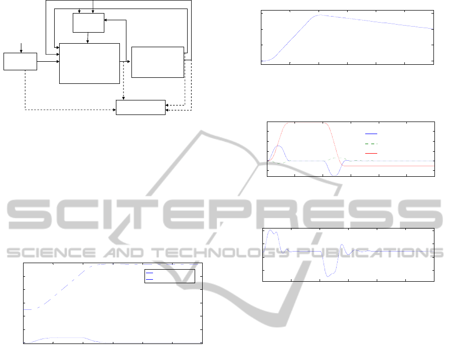
5 SIMULATOR
To predict the behaviours of the vehicle, we made a
simulator by using the dynamic model obtained from
the equation of Newton-Euler. The simulator
architecture is described in figure 5.
5.1 Direct Dynamic Model with
Constraints
To keep the tires in contact with the ground, we
must add four constraints to the dynamic model.
Therefore, the vertical velocity and acceleration of
the contact tire/road with respect to the reference
frame must be equal to zero.
[
]
0
)3(18)3(11)3(8)3(5
''''
=Φ=
a
T
ffff
qVVVV

(9)
[
]
0
)3(18)3(11)3(8)3(5
''''
=Φ+Φ=
aa
T
ffff
qqVVVV
d
t
d



(10)
Equation (13) becomes:
λ
T
mam
HqA Φ++=Γ

Where:
- λ is the lagrangien multiplier vector
- Φ
T
λ represents the vector of the efforts
transmitted by joints to respect the
constraints.
And the direct dynamical model that gives the joint
accelerations as a function of joint positions,
velocities torques, and external wrenches (forces and
moments) will be:
][
0
)(
1
)44(
mm
x
T
tm
a
H
qA
q
−Γ
⎥
⎥
⎦
⎤
⎢
⎢
⎣
⎡
Φ
Φ
=
⎥
⎦
⎤
⎢
⎣
⎡
−
λ

(11)
MODELING AND SIMULATING A NARROW TILTING CAR
233

t
q
t
q

t
q

Direct
Dynamical
Model
Integrators
+Transformation
matrix
External
Wrenches
Visualization
Trajectory
Scenario
Desired
Torques
Figure 5: Simulator architecture.
6 SIMULATION
Two scenarios are considered. In the first, the
vehicle is subject to a traction torque applied on the
rear wheels which generate an acceleration phase
then a decelerating one as shown in Figure 6. The
trajectory is a straight line with initial velocity of 5
m/s.
0 5 10 15 20 25 30
0
2
4
6
8
10
12
Time (s)
Longitudinal Velocity (m/s)
and acceleration of c.g(m/s2)
Velocity
Acceleration
Figure 6: Longitudinal velocity and acceleration of c.g.
In the second the vehicle is subject to a desired
steering torque to follow the trajectory of Figure 7.
However, to maintain the stability, the bicycle must
tilt into the corner such that the resultant force of the
lateral acceleration and the weight of the vehicle is
along the vertical axis of the vehicle (So et al 1997).
The desired tilt angle will be the roll of the bicycle
and it will be equal to:
)/(tan
1
1
gV
x
f
des
ψθ

−
=
(12)
In order to get that, a simple PD controller is
used to stabilize the roll dynamics to the desired tilt
angle (Figure 8). The controller’s output represents
the required tilting torque applied on the rear lyre to
stabilize the vehicle (Figure 9).
0 10 20 30 40 50 60
0
5
10
15
x longitudinal distance (m)
y laterral distance (m)
Figure 7: Trajectory of c.g in the horizontal plan.
0 5 10 15 20 25 30
-0.2
0
0.2
0.4
0.6
Time (s)
Roll,Yaw &
steering Angle (rd)
steering angle
Roll angle
Yaw angle
Figure 8: Trajectory of c.g in the horizontal plan.
0 5 10 15 20 25 30
1.5
1.55
1.6
1.65
Time (s)
Lyre angle (rd)
Figure 9: Rear Lyre motorized angle.
7 CONCLUSIONS
This paper presents the dynamical model of a
narrow tilting car where the structure is complex.
Future works consists on, simulating more scenarios
as high speed, considering aerodynamic forces,
elaborating robust control strategies to avoid
external perturbation and maintain the stability of
the vehicle.
REFERENCES
Karnopp, D., Fang C. 1992. Simple model of steering
controlled banking vehicles, ASME Dynamics Systems
and Control Division (DSC), 44, pp. 15-28.
Hibbard, R., Karnopp, D., 1992, The dynamics of small,
relatively tall and narrow tilting ground vehicle ASME
Dynamics Systems and Control, 52, pp. 397-417.
So, S. G., Karnopp, D., 1997, Active dual mode tilt control
for narrow ground vehicle, Vehicle System Dynamics
journal, vol 27, pp 19-36, 1997.
Hibbard, R., Karnopp, D., 1992, Optimum roll angle
behavior for tilting ground vehicles, ASME Dynamics
Systems and Control Division (DSC),vol 44, pp. 237.
ICINCO 2011 - 8th International Conference on Informatics in Control, Automation and Robotics
234

Gohl, J. and al, 2006 Development of a Novel Tilt
Controlled Narrow Commuter Vehicle, CTS,
Minnesota.
Rajamani, R., 2006, Vehicle dynamics and control,
Springer.
Kiencke., U, Nielsen, L., 2000, Automative Control
Systems for Engine, Driveline and Vehicle. New York:
Springer-Verlag.
Khalil, W., Kleinfinger, J., 1986, A new geometric
notation for open and closed loop robots, IN Proc.
IEEE on robotics and automation, pp. 1174- 1180,
San Francisco, CA, USA.
Khalil, W., Creusot D., 1997, Symoro+: A system for the
symbolic modelling of robots, Robotica, vol. 15, no. 2,
pp. 153–161.
Khalil, W. and Dombre, E., 2002, Modeling, Identification
and Control of Robots. London: Hermès Penton.
Lumeneo, www.lumeneo.fr.
Maakaroun, S., Khalil, W. and al., 2010, Geometrical
Model of a New Narrow Tilting Car, In Proc. 15th Int
Conf. on Methods and Model, in Automation and
Robotics, Miedzyzdroje, Poland.
Maakaroun, S., Khalil, W. and al., 2011, Modeling and
Simulation of a Two wheeled vehicle with suspensions
by using Robotic Formalism, In Proc. 18th IFAC
World Congress, Milan, Italy.
Gautier, M., Khalil, W., 1990, Direct calculations of
minimum set of inertial parameters of serial robots,
IEEE Trans. On Robotics and Automation, Vol. RA-
6(3), p. 368-373.
Pacejka, H. B., 2002, Tyre and Vehicle Dynamics,
Oxford, U.K.: Butterworth-Heinemann.
Canudas deWit, P and al, 2003, Dynamic friction models
for road/tire longitudinal interaction, Veh. Syst. Dyn.,
vol. 39, no. 3, pp. 189–226.
So, S., Karnopp, D., 1997, “Active dual mode tilt control
for narrow ground vehicles”, Vehicle System
Dynamics, vol. 27 pp. 19-39.
MODELING AND SIMULATING A NARROW TILTING CAR
235