TRACKING CONTROL FOR
TWO-DIMENSIONAL OVERHEAD CRANE
Feedback Linearization with Linear Observer
Tam´as R´ozsa and B´alint Kiss
Department of Control Engineering and Information Technology, Budapest University of Technology and Economics
Magyar Tud´osok krt. 2, Budapest, Hungary
Keywords:
Overhead crane, Motion planning, Tracking control, Flatness, Feedback linearization, Taylor approximation,
Linear observer.
Abstract:
A possible way to control non-linear systems is the use of exact linearization and the application of a tracking
controller to ensure exponential decay of the error along the reference trajectory. In case of overhead cranes,
it can be used if the load coordinates (or alternatively the rope angles) are known which is not the case in real
applications, where the motor axis displacements are usually measured. This paper applies the linearization
techniques such that the calculations of unmeasured states are realized with an observer, which is constructed
for the linear approximation of the dynamics along the reference trajectory. Simulation results are provided to
prove the applicability of the concept.
1 INTRODUCTION
Cranes and other types of weight handling equip-
ment are used to carry heavy loads (Gustafsson, 1996;
D. Buccieri and Bonvin, 2005; Kiss and Mullhaupt,
1999). In many cases, the load is attached to the me-
chanical structure with a rope, so the load position
cannot be directly actuated and the resulting oscilla-
tory behavior may present serious difficulties to inex-
perienced human operators. This oscillatory nature of
crane-like underactuated mechanical systems makes
them a popular benchmark application in control en-
gineering. Several tracking and sway elimination al-
gorithms are proposed in the literature (L´evine et al.,
1997; Marttinen et al., 1990; Neupert and Schneider,
2006; Overton, 1996; Hong et al., 1998), but many
of them are based on the knowledge of the load co-
ordinates (or alternatively the rope angles) which are
generally difficult to robustly measure in real applica-
tions.
The flatness property (L´evine, 2009) of the crane
models implies their feedback linearizability and it
can also be exploited for motion planning purposes.
We propose to apply a time-varying linear observer
to the linearized system dynamics along the reference
trajectory to determine the value of the unmeasured
state variables which need to be injected in the track-
ing feedback. The calculations and the simulation re-
sults will be presented on a simple, two-dimensional
overhead crane and they can be generalized for more
complex structures.
The remaining part of the paper is organized as
follows. Section 2 introduces some notations and
presents the dynamics of the two-dimensional over-
head crane. The tracking controller and the observer
design is presented in Section 3. Simulation results
of the trajectory behavior are shown in Section 4, and
our results are summarized in Section 5.
2 SYSTEM DYNAMICS
The two-dimensional overhead crane is illustrated in
Figure 1. The horizontal displacement of the cart with
mass M is denoted by R. The cart is actuated by a
motor delivering the force F which is considered to
be one of the input of the dynamics. The load with
mass m, having the coordinates (x
m
,z
m
) is accelerated
through a rope with the length of L, winched on a
drum of inertia J and radius ρ with a motor delivering
the torque T. The angle between the rope and the
vertical is denoted by θ. We assume no friction and
massless rope and due to the small value of ρ, we also
assume that the rope always connects to the winch at
point (R+ρ, 0). The resulting mechanical system has
427
Rózsa T. and Kiss B..
TRACKING CONTROL FOR TWO-DIMENSIONAL OVERHEAD CRANE - Feedback Linearization with Linear Observer.
DOI: 10.5220/0003539604270432
In Proceedings of the 8th International Conference on Informatics in Control, Automation and Robotics (ICINCO-2011), pages 427-432
ISBN: 978-989-8425-74-4
Copyright
c
 2011 SCITEPRESS (Science and Technology Publications, Lda.)



















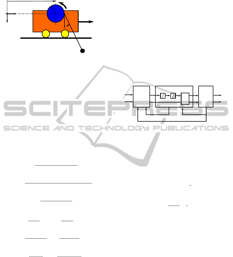
Figure 1: The overhead crane.
three degrees of freedom so the dimension of the state
vector x is six. Several possible choices exist for x.
The non-linear system dynamics can be written in
the classical form (Isidori, 1995):
˙x = f(x) + g(x)u (1)
where x and u denote the state and input vectors, re-
spectively. Let us define
x =
h
R
˙
R
θ
˙
θ
L
˙
L
i
T
(2)
u =
h
F T
i
T
(3)
such that f and g read
f(x) =













˙
R
mJL
˙
θ
2
sinθ+mgJsinθcosθ
D
˙
θ
−
sinθ(Dg+mJL
˙
θ
2
cosθ)+mgJcos
2
θ+2D
˙
L
˙
θ
LD
˙
L
mMρ
2
(L
˙
θ
2
+gcosθ)
D













(4)
g(x) =













0 0
mρ
2
+J
D
mρsinθ
D
0 0
−
cosθ(mρ
2
+J)
LD
−
mρsinθcosθ
LD
0 0
−
mρ
2
sinθ
D
−
ρ
(
msin
2
θ+M
)
D













(5)
with
D = D(θ) = mMρ
2
+ mJsin
2
θ+ MJ. (6)
3 TRACKING CONTROL
In this section we present the linearizing and the
tracking controller first, then we give the details of
the observer design steps.
3.1 Stabilizing Feedback
It has been shown in (Fliess et al., 1993; L´evine et al.,
1997; Kiss and Mullhaupt, 1999) that the system
(1)–(5) with output
y =


h
1
(x)
h
2
(x)


=


R+ ρ + Lsinθ
Lcosθ


(7)
is differentially flat, which implies that the model is
feedback linearizable. The conception is shown in
Figure 2. Notice that the elements of the flat out-
put have been chosen as the Cartesian coordinates
(x
m
,z
m
) of the load.













 


 



!


!

"



Figure 2: Block diagram of the linearizing feedback.
Based on (Boustany and d’Andr´ea Novel, 1992),
the equations of the dynamic compensator are


F
T


= α(x) + β(x)


ξ
v
2


(8)
α(x) =


−mgsinθcosθ
mgρcosθ−
J
ρ
L
˙
θ
2


(9)
β(x) =


msinθ M
−
mρ
2
+J
ρ
J
ρ
sinθ


(10)
¨
ξ = v
1
(11)
Notice that ξ is the tension in the rope, divided by the
load mass.
Combining (1)–(6) and (8)–(11), the extended
state-space model can be written in the form
˙
˜x =
˜
f( ˜x) +
h
˜g
1
( ˜x) ˜g
2
( ˜x)
i
˜u (12)
with the new state and input vectors
˜x =
h
R
˙
R θ
˙
θ L
˙
L ξ
˙
ξ
i
T
(13)
˜u =
h
v
1
v
2
i
T
(14)
In fact, the new vector fields
˜
f, ˜g
1
, ˜g
2
read
ICINCO 2011 - 8th International Conference on Informatics in Control, Automation and Robotics
428

˜
f( ˜x) =



















˙
R
0
˙
θ
−2
˙
L
˙
θ−gsinθ
L
˙
L
L
˙
θ
2
+ ξ
˙
ξ
0



















(15)
˜g
1
( ˜x) =



















0
0
0
0
0
0
0
1



















˜g
2
( ˜x) =



















0
1
0
−
cosθ
L
0
− sinθ
0
0



















(16)
This extended model can be exactly linearized with
static feedback which has the form (Isidori, 1995):


v
1
v
2


= A
−1
( ˜x) ·




x
(4)
m
z
(4)
m


− b( ˜x)


(17)
where A and b are calculated via Lie derivatives:
A( ˜x) =


L
˜g
1
L
3
˜
f
h
1
L
˜g
2
L
3
˜
f
h
1
L
˜g
1
L
3
˜
f
h
2
L
˜g
2
L
3
˜
f
h
2


(18)
b( ˜x) =


L
4
˜
f
h
1
L
4
˜
f
h
2


(19)
The resulting system is a decoupled linear system
˙x
′
= A
′
x
′
+ B
′
u
′
(20)
with
x
′
=
h
x
m
˙x
m
¨x
m
x
(3)
m
z
m
˙z
m
¨z
m
z
(3)
m
i
T
(21)
u
′
=
h
x
(4)
m
z
(4)
m
i
T
(22)
The elements of the new state vector x
′
can be ex-
pressed in coordinates of ˜x in (13). Note that the dif-
feomorphism is singular if
cosθ(gcosθ− ξ) = 0 (23)
One can easily design an additional feedback law for
the linear dynamics (20) which ensures the exponen-
tial decay of the tracking error, so that
e
(4)
x
+ k
x,3
e
(3)
x
+ k
x,2
¨e
x
+ k
x,1
˙e
x
+ k
x,0
e
x
= 0 (24)
e
(4)
z
+ k
z,3
e
(3)
z
+ k
z,2
¨e
z
+ k
z,1
˙e
z
+ k
z,0
e
z
= 0 (25)
are satisfied where
e
x
= x
m,ref
− x
m
(26)
e
z
= z
m,ref
− z
m
(27)
To determine the coefficients k
x,i
, k
z,i
, i = 0,1, 2,3,
several methods can be used, e.g., LQR and pole
placement techniques (Brogan, 1990).
3.2 State Observer
The previously proposed method assumes that the
state vector x in (2) is known. However, in real appli-
cations only motor positions can be easily measured,
i.e., R and L, but θ is difficult to determine.
We apply a linear state observer (Brogan, 1990)
for this purpose, calculating the first-order Taylor ap-
proximation of the non-linear model (1)–(5) for every
timestep along track. Simulationresults show that this
technique gives satisfactory result (see Section 4).
Introducing
¯x = x− x
0
(28)
¯u = u− u
0
(29)
¯y = y− y
0
(30)
the linear approximation of (1)–(5) at (x
0
, u
0
) can be
written as follows:
˙
¯x =
¯
A(x
0
,u
0
) ¯x+
¯
B(x
0
,u
0
) ¯u (31)
The matrices
¯
A and
¯
B are calculated via symbolic
derivation:
¯
A =
∂f(x,u)
∂x



(x
0
,u
0
)
(32)
¯
B =
∂f(x,u)
∂u



(x
0
,u
0
)
(33)
One can design a linear observer in the form
˙
ˆ
¯x =
¯
F(x
0
,u
0
)
ˆ
¯x +
¯
G(x
0
,u
0
) ¯y+
¯
H(x
0
,u
0
) ¯u (34)
where
ˆ
¯x denotes the estimation of ¯x, and
¯
F,
¯
G,
¯
H can
be chosen such that the estimation error ¯x−
ˆ
¯x decays
exponentially.
Since the matrices
¯
A,
¯
B,
¯
F,
¯
G,
¯
H depend on the op-
erating point, they are time-varying. Nevertheless,
they can be calculated off-line for every reference tra-
jectory which is important in real-time applications.
Note that this method also enables to design an
additional load estimator which ensures robustness
against unknown disturbances on the system input
channels, i.e., F and T. Laboratory experiments show
that this is an effective way to cancel friction forces.
TRACKING CONTROL FOR TWO-DIMENSIONAL OVERHEAD CRANE - Feedback Linearization with Linear
Observer
429

3.3 Motion Planning
It is expected to carry the load with zero velocity
and acceleration in the initial and final positions, so
any oscillations in these two points are to be avoided.
One can easily design a reference trajectory based on
polynomial approximation, which satisfies these con-
straints (L´evine, 2009).
In the two-dimensional overhead crane example,
the following expression can be used to calculate the
reference trajectory in x direction:
x
m
(t) = x
m,I
+ (x
m,F
− x
m,I
) ·
9
∑
i=5
a
i

t − t
I
t
F
− t
I

i
(35)
where t ∈ [t
I
,t
F
] and t
I
, t
F
denotes the time at the ini-
tial and final positions, respectively. The coefficients
a
i
are computed by solving a system of linear equa-
tions produced by the constraints mentioned above,
namely x
m
(t
I
) = x
m,I
, ˙x
m
(t
I
) = ¨x
m
(t
I
) = x
(3)
m
(t
I
) =
x
(4)
m
(t
I
) = 0 and x
m
(t
F
) = x
m,F
, ˙x
m
(t
F
) = ¨x
m
(t
F
) =
x
(3)
m
(t
F
) = x
(4)
m
(t
F
) = 0 In fact, the numerical values
of the coefficients are
a
5
= 126 a
6
= −420
a
7
= 540 a
8
= −315
a
9
= 70
(36)
The derivatives can be easily calculated as well. The
method in z direction is exactly the same as presented
for x.
There are some situations, for example if an ob-
stacle is present in the crane’s workspace, when other
type of path is required. According to (L´evine, 2009),
the geometry of the trajectory can be given by the
function
z
m
= z
m
(x
m
) (37)
where x
m
= x
m
(t) can be calculated using the polyno-
mial interpolation described by (35). Moreover, the
geometry can also be specified in the following form:
x
m
= x
m
(λ) (38)
z
m
= z
m
(λ) (39)
Here λ = λ(t) denotes the path parameter which can
also be calculated using (35).
4 SIMULATIONS
This section shows simulation results based on the
methods described above. The parameters are given
as follows: m = 1kg, M = 3kg, J = 0.1kgm
2
,
ρ = 1.5cm, x
m,I
= 0.1m, z
m,I
= 1.1m, x
m,F
= 1.1m,
z
m,F
= 0.1m, T = 2s; sample time is set to 0.001s and
  




 
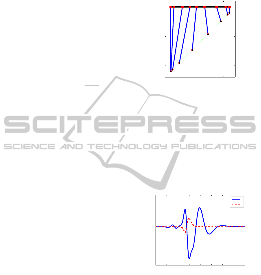
Figure 3: Illustration of the desired behavior.
the reference path is a straight line with a length of
1.41m. It is illustrated in Figure 3. Using pole place-
ment technique, the observer’s poles have been placed
equidistantly between −5 and −15, while the closed-
loop poles have been placed with the outer-loop con-
troller to −5.
In the first simulation the model was initialized
with the values of the reference trajectory. In this
case, Figure 4 shows the differences between the real
and estimated positions. One can see that the absolute
value of the highest error is 10
−4
m, which is totally
acceptable in most cases.
        











Figure 4: Estimation error in x and z directions.
On the other hand, if the initial states of the
crane model differ from the reference states, the
controller is still able to stabilize the system. Let
us consider some initial oscillation, i.e., θ
I
= π/20,
˙
θ
I
= −0.5rad/s. Theposition errorsareshown in Fig-
ure 5. The observer produces greater error here than
in the previous case, but the system still reaches the
equilibrium. Notice that initial error is also present
since the estimator starts from the reference initial
states.
Finally, Figure 6 shows the case when the ini-
ICINCO 2011 - 8th International Conference on Informatics in Control, Automation and Robotics
430

        








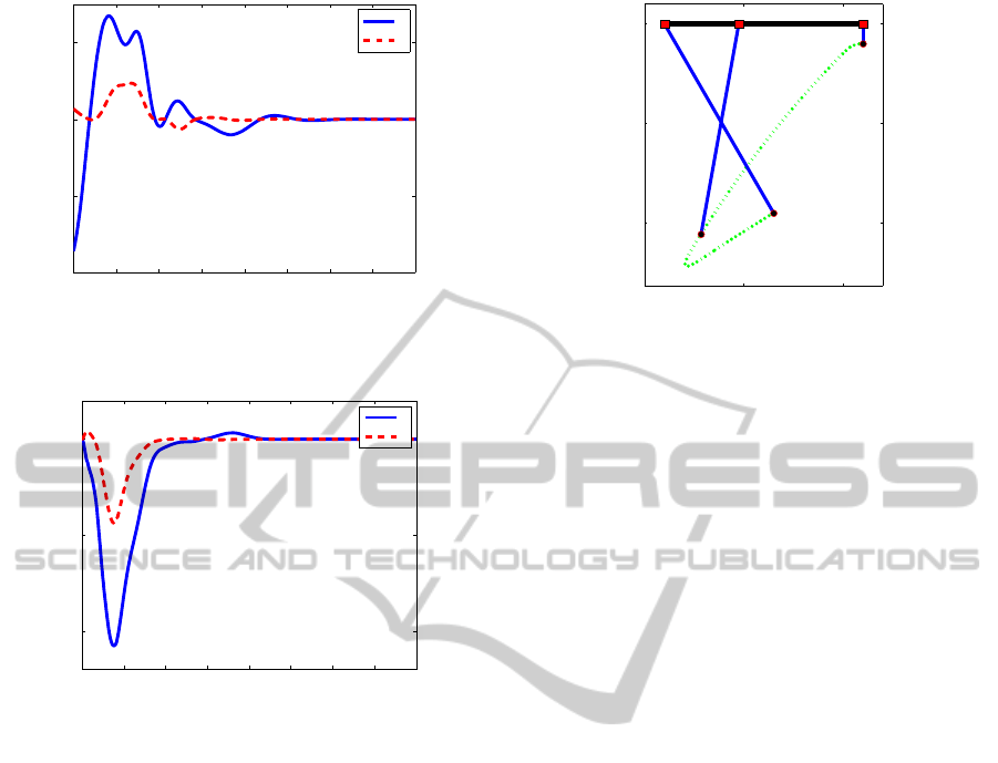
Figure 5: Estimation error in x and z directions if the crane
model starts with an initial trajectory error.
        







Figure 6: Estimation error in x and z directions if both the
model and the observer start with the same initial state,
which is not the initial reference state.
tial states of the crane model differ from the refer-
ence states, but the observer’s states are also set to the
model’s initial states. It means that the initial error
is known so the observer can be initialized properly.
Thus, the initial estimation error is zero in this case.
The states have been modified to θ
I
= π/6,
˙
θ
I
=
−1rad/s. Although the load starts far from the ref-
erence path (in fact, the distance is 0.57m), the con-
troller stabilizes the system and the load is taken to
the desired location. Figure 7 illustrates the trajectory
in this situation.
5 CONCLUSIONS
We have presented the tracking controlproblem of the
two-dimensional overhead crane. A general approach
to solve it is using feedback linearization. It requires
the exact knowledge of the system states, however,
usually only two of the six states are measured. We
proposed a simple estimation method to calculate the
unmeasured states, which is based on the Taylor ap-
  




 
Figure 7: Trajectory in the case of high initial error.
proximation of the non-linear crane model. Simula-
tion results show that this approach gives satisfactory
result for small errors. Further research on this topic
might include stability analysis with parameter uncer-
tainties, and application to a laboratory equipment.
ACKNOWLEDGEMENTS
This work is connected to the scientific program of
the ”Development of Quality-Oriented and Harmo-
nized R+D+I Strategy and FunctionalModel at BME”
project. This project is supported by the New Hun-
gary Development Plan (Project ID: TMOP-4.2.1/B-
09/1/KMR-2010-0002). The work is partially sup-
ported by the Hungarian Scientific Research Fund un-
der grant OTKA K71762.
REFERENCES
Boustany, F. and d’Andr´ea Novel, B. (1992). Adaptive
control of an overhead crane using dynamic feedback
linearization and estimation design. In Robotics and
Automation, 1992. Proceedings., 1992 IEEE Interna-
tional Conference on, pages 1963–1968 vol.3.
Brogan, W. L. (1990). Modern Control Theory (3rd Edi-
tion). Prentice Hall.
D. Buccieri, P. M. and Bonvin, D. (2005). Spider-
carne: Model and properties of a fast weight handling
equipment. In Proceedings of the 16th IFAC World
Congress.
Fliess, M., L´evine, J., and Rouchon, P. (1993). A gen-
eralised state variable representation for a simplified
crane description. Int. J. of Control, 58:277–283.
Gustafsson, T. (1996). On the design and implementation
of a rotary crane controller. European J. Control,
2(3):166–175.
TRACKING CONTROL FOR TWO-DIMENSIONAL OVERHEAD CRANE - Feedback Linearization with Linear
Observer
431

Hong, K., Kim, J., and Lee, K. (1998). Control of a con-
tainer crane: Fast traversing, and residual sway con-
trol from the perspective of controlling an underactu-
ated system. In Proceedings of the ACC, pages 1294–
1298, Philadelphia, PA.
Isidori, A. (1995). Nonlinear Control Systems. Springer.
Kiss, B., L. J. and Mullhaupt, P. (1999). Modeling, flat-
ness and simulation of a class of cranes. Periodica
Polytechnica-Electrical Engineering, 43(3):215–225.
L´evine, J. (2009). Analysis and Control of Nonlinear Sys-
tems. Springer.
L´evine, J., Rouchon, P., Yuan, G., Grebogi, C., Hunt, B.,
Kostelich, E., Ott, E., and Yorke, J. (1997). On the
control of US navy cranes. In Proceedings of the Eu-
ropean Control Conference, pages N–217, Brussels,
Belgium.
Marttinen, A., Virkkunen, J., and Salminen, R. (1990).
Control study with a pilot crane. IEEE Trans. Edu.,
33:298–305.
Neupert, J., H. A. S. O. and Schneider, K. (2006). Trajec-
tory tracking for boom cranes using a flatness based
approach. In Proceedings of the SICE-ICASE Inter-
national Joint Conference, pages 1812–1816.
Overton, R. (1996). Anti-sway control system for cantilever
cranes. United States Patent, (5,526,946).
ICINCO 2011 - 8th International Conference on Informatics in Control, Automation and Robotics
432