VALIDATED MODEL OF A PRESSURE MICROPROBE FOR
WATER RELATIONS OF PLANT CELLS
Victor Bertucci-Neto and Paulo Estevão Cruvinel
Embrapa Instrumentação Agropecuária, Rua XV de Novembro, 1452,13560-970, São Carlos, SP, Brazil
Keywords: Model vegetable cell, Pressure probe, Instrument turgor.
Abstract: Turgor pressure is a physiologic variable of fundamental importance. It is a component of water potential
and a measure of water status in a plant. For a long time direct measurement of turgor pressure was not
possible. Three decades ago a pressure probe technique was originally introduced to measure turgor
pressure and water relations of higher plant cells. Early experiments were made with a glass capillary linked
to a pressure chamber, filled with silicone oil. After the vegetable cell to be punctured with the tip of the
capillary, a sensor was used to measure the pressure in the chamber. From then until now the usual
procedure has been to detect the meniscus position at the moment that the cell is punctured and manually, or
automatically, to return the meniscus to the original position. When this occurs the pressure in the chamber
is measured with a sensor. Some attempts were made to get the instrument automated but there is no
systematic description about it. Based on this, it is proposed a dynamic model for the hydraulic system that
can be helpful to design a closed loop system aiming an automated instrument. It is also shown that the
theoretical model reasonably matches the experimental results.
1 INTRODUCTION
Turgor pressure is a physiologic variable of
fundamental importance. It is a component of water
potential and a measure of water status in a plant.
For mature, turgid cells of higher plants, changes of
water potential are largely reflected in changes of
turgor. For a long time, the direct measurement of
turgor was not possible (Steudle, 1993). Three
decades ago a pressure probe technique was
originally introduced to measure turgor and water
relations of higher plant cells (Husken et al., 1978).
Early experiments were made with a glass capillary
linked to a pressure chamber, filled with silicone oil.
After the vegetable cell to be punctured with the tip
of the capillary, a sensor was used to measure the
pressure in the chamber. Later, it was remarked that
a necessary condition for constructing cell pressure
probes is given by:
inol
ol
Vc
B
V
>>
(1)
where V
ol
and V
in
are the internal volumes of the cell
and apparatus respectively, B is the elastic
coefficient of the cell, and c
ol
is the coefficient of
compressibility of the oil. The condition imposed by
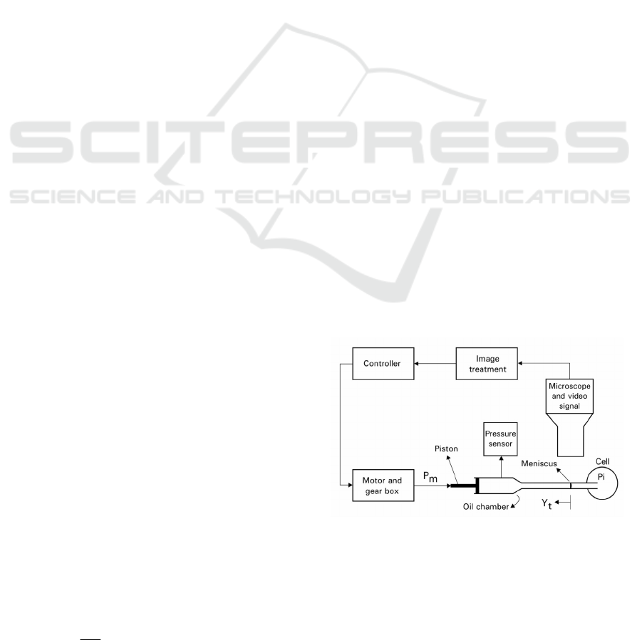
Figure 1: Schematic diagram of a pressure microprobe.
Equation (1) indicates that V
in
must be reduced in
several orders of magnitude, and the meniscus
formed at the tip of the capillary must be used as a
reference of measurement. From then to now the
usual procedure has been to detect the meniscus
position at the moment that the cell is punctured
manually, or automatically, to return the meniscus to
the original position. When this occurs the pressure
in the chamber is measured with a sensor. In the
Figure 1 is shown a schematic diagram representing
433
Bertucci-Neto V. and Estevão Cruvinel P..
VALIDATED MODEL OF A PRESSURE MICROPROBE FOR WATER RELATIONS OF PLANT CELLS.
DOI: 10.5220/0003539704330436
In Proceedings of the 8th International Conference on Informatics in Control, Automation and Robotics (ICINCO-2011), pages 433-436
ISBN: 978-989-8425-74-4
Copyright
c
2011 SCITEPRESS (Science and Technology Publications, Lda.)

the pressure probe acting on a cell, with the
meniscus being observed by the microscope and
video camera. After the image treatment, the signal
equivalent to the meniscus position is sent to the
controller. The controller acts on the motor and
reducing gear causing the movement of the piston
returning the meniscus to the original position. Some
attempts were made to get the instrument automated
(Husken et al., 1978, and Cosgrove and Durachko,
1986) but there is no systematic description about it.
Manual measurements can be made during short
times but it can be difficult if one wants to register
long term behaviour. Moreover, manual operation is
based on the operator skill and in the subjective
interpretation of the image. By the other hand,
control system algorithms can be more easily
designed and implemented when the system plant is
reasonably known. Based on this, it is proposed a
dynamic model for the hydraulic system that can be
helpful to design a closed loop system aiming an
automated instrument. In addition, the mathematical
model can be useful to understand the contribution
of each physical parameter to the measurement
performance.
2 SYSTEM MODELLING
The system modelling is based on the analysis of
pipe flow. It is considered a cylindrical element
(radius=r, and length=L) in a pipeline and expressed
the loss in pressure due to the forces acting on the
fluid. Balancing the forces in terms of the pressure p
along the longitudinal axis y, including the retarding
force due to the shear stress τ
w
gives:
()
[]
()()
dyrrdppp
w
πτπ
2
2
=+−
(2)
resulting in:
dy
r
dp
w
τ
2
=−
(3)
Integrating both sides of Equation (3) from the
pressure at the downstream end to the upstream end,
and along the length of the element, yields the
amount in pressure Δp that droped:
L
r
p
w
τ
2
=Δ
(4)
Last equation shows the relation between shear
stress and the pressure drop. Δp can be equated to
the specific weight γ=ρg (density multiplied by
gravity acceleration) multiplied by the heading loss
h
L
. Then Equation (4) can be rewritten:
r
L
h
L
w
2
γ
τ
=
(5)
In the case of laminar flow in the pipe Newton’s law
of viscosity can be written as τ
w
being proportional
to the velocity gradient v related to the radius, with
constant of proportionality defined as the coefficient
of viscosity μ. Then Equation (5) can be written:
dr
dv
r
L
h
L
w
μ
γ
τ
−==
2
(6)
Integrating last equation from the maximum velocity
v
c
(at the center of the pipe) to v, and from 0 to r,
becomes:
2
4
r
L
h
vv
L
c
μ
γ
−=
(7)
Last equation shows that the velocity profile is a
parabolic curve. When r=0, v=v
c
. Substituting v=0,
and r=d
t
/2 (d
t
is the tube diameter), and considering
v
c
=2V, being V the mean velocity, then:
2
32
t
L
d
LV
h
γ
μ
=
(8)
showing that the head loss is proportional to the
mean velocity. By setting Equation (8) equal to
Darcy’s equation (Vennard, 1961) it can be derived
an expression for the friction factor for laminar pipe
flow:
ρ
μ
t
Vd
f
64
=
(9)
By the other hand, multiplying both sides of Darcy’s
equation by
γ
=
ρ
g and equating to the same pressure
drop h
L
γ
obtained in Equation (5):
8
4
2
22
V
f
d
LV
d
L
fhp
w
t
w
t
L
ρττργ
=⇒===Δ
(10)
Using the friction factor given in the Equation (9)
and substituting in the last equation it is obtained an
expression that relates the shear stress to the
velocity, or:
t
w
d
V
μ
τ
8
=
(11)
The analysis that follows is described in Doebelin
(1990) that considered a gas system with tube
ICINCO 2011 - 8th International Conference on Informatics in Control, Automation and Robotics
434

volume a small fraction of chamber volume.
However the flow considered here is liquid causing
a simplification because the spring effect that exists
due to the gas flow is negligible in liquid flow case.
Analysis consists of applying Newton’s law by
balancing the forces along the tube in the
longitudinal axis y. Initially is considered that
p
m
=p
i
=p
0
(p
0
an initial arbitrary value) when p
i
changes slightly in some way. Then it is considered
at this point that p
i
and p
m
mean the excess pressures
over and above p
0
. The force f
i
due to the pressure p
i
is given by:
i
t
ii
p
d
Apf
4
2
π
==
(12)
The viscous force f
v
due to the wall shearing stress is
given by the division of Equation (11) by the area of
the pipe wall:
tv
yLVLf
πμπμ
88 ==
(13)
where y
t
is the liquid displacement due to p
i
action.
This displacement causes a volume change
dV
ol
=πd
t
2
y
t
/4 and pressure excess p
m
=πBd
t
2
y
t
/(4V
ol
)
(B is the elastic coefficient). The equivalent force is
given by:
ol
tt
m
V
yBd
f
16
42
π
=
(14)
Applying Newton’s law along the longitudinal axis
implies to balance the forces and equate to the fluid
mass m multiplied by the acceleration a, or:
amfff
mvi
⋅
=
−−
(15)
Above equation is useful for uniform velocity
distribution. However, the quadratic velocity profile
verified in Equation (7) indicates that a correction
factor must be used in the right side of Equation
(15). In this case the quantity m.a must be multiplied
by 4/3. Then, Equation (15) can be rewritten as:
t
t
t
ol
t
ti
t
y
Ld
y
V
Bd
yLp
d
316
8
4
2
42
2
ρπ
π
πμ
π
=−−
(16)
Applying Laplace transform in Equation (16) yields:
()
()
()
ol
VL
t
Bd
S
t
d
S
L
sP
sY
sG
i
t
yp
ρ
π
ρ
μ
ρ
16
2
3
2
24
2
4
3
++
==
(17)
Last equation relates the displacement of the
meniscus due to the pressure applied at the tip of the
capillary. Moreover, it permits an evaluation of the
dynamical behaviour by the variation of its physical
parameters.
3 EXPERIMENTAL SET UP AND
COMPARISON
The meniscus was observed with a video camera
coupled to a microscope. The video signal was
sampled at 70 ms and digitalized with a video board
installed in the personal computer. It was developed
a software based on Imaq Vision for LabView for the
meniscus detection. This software is based on
pattern recognition and gives as result the number of
pixels (Npixel) concerning to the previously chosen
initial position. It was coupled a “T” connection at
the tip of the capillary. The capillary was previously
filled with silicone oil. It was linked at one of the
inputs of the T connection an air duct supplied by an
air compressor. At the other input was coupled a
pressure sensor with reading rate equal to 10mV/psi.
After the air compressor to be switched on, the
readings of both meniscus position, and voltage
signal due to the sensor were collected and stored in
the computer. In the Figure 2 is shown the curve due
to the meniscus displacement (in Npixel) and the
curve due to the voltage signal in the pressure
sensor. It can be seen in Equation (17) that the final
value is L/B. This means that if the length L is
increased then the meniscus displacement is also
increased. It was used the following values for each
physical parameter in the Equation (17), with B, µ,
and ρ being attributed to the silicone oil, and L
chosen according to the optical resolution: L=0.15m;
d
t
=270 10
-6
m; ρ=900 Kg/m
3
;
B=2.18 10
9
N/m
2
;
μ=10
-3
Kg/m s. Substituting the above values results
in:
72
6
10.074.88.365
10556.5
)(
+⋅+
⋅
=
−
ss
sG
yp
(18)
To compare the mathematical model to the
experimental response it is necessary to transform
the pressure sensor signal measured in volt in
pressure dimension. Then, the voltage signal must be
multiplied by (1/0.6mV) x psi, with 1psi=6894.6
N/m
2
. The relation between the meniscus
displacement in meter and Npixel was previously
measured with a rule adapted in the microscope lens.
It was found 1 pixel=1/6.36x10
5
m. Applying the
transformed input pressure signal to the Equation
VALIDATED MODEL OF A PRESSURE MICROPROBE FOR WATER RELATIONS OF PLANT CELLS
435
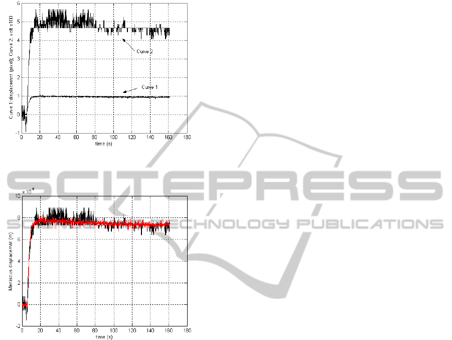
(18) results in the red curve showed in Figure 3. This
same figure shows the experimental curve.
Figure 2: Curve 1: meniscus displacement (Npixel). Curve
2: pressure sensor signal (volt x 100).
Figure 3: Meniscus displacement: experimental response
(black), and theoretical response (red).
4 CONCLUSIONS
Despite the noisy signal imposed by the meniscus
detection (mean=0.47 Npixel and variance=0.10
Npixel
2
) it can be seen in Figure 3 the strong
accordance between the theoretical and experimental
responses. The mathematical model could match the
dynamical behaviour and the steady state exhibited
in the experimental response. It was not considered
in the modelling the effects of the surface tension
and the glass compressibility because the magnitude
of both of them were previously known as
negligible. Experimental results show that the
proposed model can be applied in open and closed
loop designs according to the operation needs
(manual or automated). The modelling is also
justified in the evaluation of the contribution of each
physical parameter to the system response. This
permits to predict the importance of using high or
low viscosity silicone oil, a long or short pipe, or the
more or less compressible oil. All of these
considerations will be related to the system range
and performance.
ACKNOWLEDGEMENTS
This work was supported by Embrapa.
REFERENCES
Bertucci-Neto, V. 2005. Modelagem e automação em nova
técnica de medida para relações de água e planta.
Thesis (in portuguese). Escola de Engenharia de São
Carlos, Universidade de São Paulo. São Carlos.
Cosgrove, D. J.; Durachko, D. M. 1986. Automated
pressure probe for measurement of water transport
properties of higher plant cells. Review of Scientific
Instrument. v.57. n.10. p.2614-2619.
Doebelin, E. O. 1990. Measurement systems application
and design. 4. ed. New York: McGraw-Hill Publishing
Company.
Husken, D.; Steudle, E.; Zimmermann, U. 1978. Pressure
probe technique for measuring water relations of cells
in higher plants. Plant Physiology. v. 61. p. 158-163.
Steudle, E. 1993. Pressure probe technique: basic
principles and application to studies of water and
solute relations at the cell, tissue and organ level. Ed.
J. A. C. Smith and H. Griffiths . Oxford, UK: Bios
Scientific Publishers Ltd. p.5-36.
Vennard, J. K. (1961). Elementary fluid dynamics. 4. ed.
New York: John Wiley and Sons, Inc.
ICINCO 2011 - 8th International Conference on Informatics in Control, Automation and Robotics
436
