PRINCIPAL COMPONENTS ANALYSIS METHOD
APPLICATION IN ELECTRICAL MACHINES DIAGNOSIS
J. F. Ramahaleomiarantsoa, N. Heraud
Université de Corse, U.M.R. CNRS 6134 SPE, BP 52, 20250 Corte, France
E. J. R. Sambatra
Institut Supérieur de Technologie, BP 509, 201 Antsiranana, Madagascar
J. M. Razafimahenina
Ecole Supérieure Polytechnique, BP O, 201 Antsiranana, Madagascar
Keywords: Diagnosis, Principal components analysis, Residues, Wound rotor induction machine, Modeling.
Abstract: Electrical machines are found in many applications, especially in wind energy conversion chain (WECC).
However, these machines still remain the most potential of failures. Many researches and improvements
have been carried out but in the aim of optimal operation systems, monitoring and diagnosis techniques are
among the interests of existing laboratories and research teams. This paper deals with the principal
components analysis (PCA) method application in electrical machines, especially a wound rotor induction
machine (WRIM), diagnosis. The used PCA approach is based on residues analysis. To perform the matrix
data needed for PCA method data input, an accurate analytical method of the WRIM is proposed. WRIM
and PCA models are implemented in Matlab software. The simulation results show the potential necessity
of the considered PCA method on the WRIM faults detection compared to some other signal analysis
method.
1 INTRODUCTION
Since many years, faults detection in electrical
machines has been object of both industrial and
teaching laboratories. Previously, DC and
synchronous machines were the most used on
industry applications, and reliability researches were
focused on these types of machines. With
technological developments, power electronic
progress and the economic issue, the squirrel cage
and the wound rotor induction machines have taken
their place in several applications domain like
transportation, energy production and electrical
drives through their robustness, reliability and lower
costs. Although researches and improvements have
been carried out, these machines still remain the
most potential of the stator and the rotor failures.
In fact, this article shows one of several
methodology for monitoring and doing diagnostics
related to the faults on a wound rotor induction
machine (WRIM) based WECC by the residues
analysis of its state variables. The approach is based
on the principal components analysis (PCA) method.
The first part of this paper deals with the WRIM
modeling followed by some reminders of the
different types of stator and rotor WRIM faults. The
second part is devoted at the PCA principle. The
PCA model construction method and the choice
criterion of the number of components to be retained
is discussed, followed by the PCA residues
generation technical for the faults detection and the
localization. The third part talks about the method
validations using Matlab/Simulink software. The
simulation results of several variables (stator and
rotor currents, shaft rotational speed, electrical
power, electromagnetic torque and other variables
issued from mathematical transformations) of
healthy and faulted WRIM are analyzed.
167
F. Ramahaleomiarantsoa J., Heraud N., J. R. Sambatra E. and M. Razafimahenina J..
PRINCIPAL COMPONENTS ANALYSIS METHOD APPLICATION IN ELECTRICAL MACHINES DIAGNOSIS.
DOI: 10.5220/0003542501670175
In Proceedings of the 8th International Conference on Informatics in Control, Automation and Robotics (ICINCO-2011), pages 167-175
ISBN: 978-989-8425-74-4
Copyright
c
 2011 SCITEPRESS (Science and Technology Publications, Lda.)

Special attention has been reserved to the PCA
residues representations. The last part is reserved to
the analyze and discussion of simulation results.
2 WRIM MODELLING
In the process of faults survey and diagnosis, an
accurate modeling of the machine is necessary. In
this paper, three phases model based on
magnetically coupled electrical circuits was chosen.
The aim of the modeling is to highlight the
electrical faults influences on the different state
variables of the WRIM. For that, some modeling
assumptions given in the following section are
necessary.
2.1 Modeling Assumptions
In the proposed approach, we assumed that:
• the magnetic circuit is linear, and the relative
permeability of iron is very large compared to the
vacuum.
• the skin effect is neglected,
• hysteresis and eddy currents are neglected,
• the airgap thickness is uniform,
• magnetomotive force created by the stator and the
rotor windings is sinusoidal distribution along the
airgap,
• the stator and the rotor have the same number of
turns in series per phase,
• the coils have the same properties,
• the WRIM stator and rotor coils are coupled in star
configuration and connected to the considered
balanced state grid.
2.2 Differential Equation System of the
WRIM
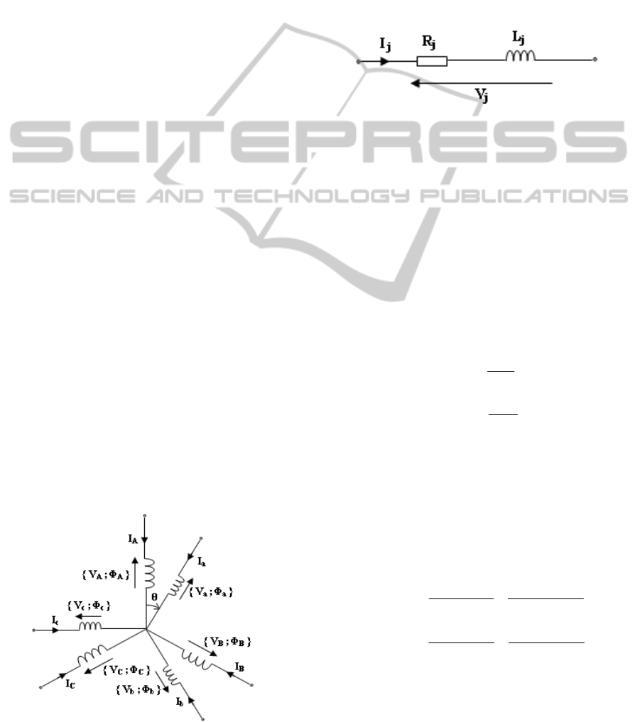
Figure 1: Equivalent electrical circuit of the WRIM.
V
j
, I
j
and Φ
j
(j : A, B, C for the stator phases et a, b,
c, for the rotor phases) are respectively the voltages,
the electrical currents and the magnetic flux of the
stator and the rotor phases, θ is the angular position
of the rotor relative to the stator.
The figure 1 shows the equivalent electrical
circuit of the WRIM. Each coil, for both the stator
and the rotor, is modelised with a resistance and an
inductance connected in series configuration (Fig.
2).
Figure 2: Equivalent electrical circuit of the WRIM coils.
We note the voltages vector ([V
S
], [V
R
]), the
currents vector ([I
S
], [I
R
]) and the flux vector ([Φ
S
],
[Φ
R
]) of respectively the stator and the rotor:
[]
⎥
⎥
⎥
⎦
⎤
⎢
⎢
⎢
⎣
⎡
=
C
B
A
S
V
V
V
V
;
[]
⎥
⎥
⎥
⎦
⎤
⎢
⎢
⎢
⎣
⎡
=
C
B
A
S
I
I
I
I
;
[]
⎥
⎥
⎥
⎦
⎤
⎢
⎢
⎢
⎣
⎡
=
C
B
A
S
φ
φ
φ
φ
[]
⎥
⎥
⎥
⎦
⎤
⎢
⎢
⎢
⎣
⎡
=
c
b
a
R
V
V
V
V
;
[]
⎥
⎥
⎥
⎦
⎤
⎢
⎢
⎢
⎣
⎡
=
c
b
a
R
I
I
I
I
;
[]
⎥
⎥
⎥
⎦
⎤
⎢
⎢
⎢
⎣
⎡
=
c
b
a
R
φ
φ
φ
φ
[][][]
[]
dt
d
IRV
S
SSS
φ
+=
(1)
[][][]
[]
dt
d
IRV
R
RRR
φ
+=
(2)
[
]
[
]
[
]
[
][ ]
RSRSSS
IMIL
+
=
φ
(3)
[
]
[
]
[
]
[
][ ]
SRSRRR
IMIL
+
=
φ
(4)
[R
S
] and [R
R
] are the resistances matrix, [L
S
] and [L
R
]
the own inductances matrix, and [M
SR
] and [M
RS
] the
mutual inductances matrix between the stator and
the rotor coils.
With (3) and (4), (1) and (2) become:
[][][]
[
]
[
]
{
}
[][]
{}
dt
IMd
dt
ILd
IRV
RSRSS
SSS
++=
(5)
[][][]
[
]
[
]
{
}
[][] {}
dt
IMd
dt
ILd
IRV
SRS
RR
RRR
++=
(6)
By applying the fundamental principle of dynamics
to the rotor, the mechanical motion equation is
(Wieczorek and Rosołowski, 2010):
ICINCO 2011 - 8th International Conference on Informatics in Control, Automation and Robotics
168

remvt
CCf
dt
d
J −=Ω+
Ω
(7)
dt
d
θ
=Ω
(8)
with:
[]
[
]
(
)
[]
I
d
Ld
IC
t
em
* *
2
1
θ
=
(9)
t
J is the total inertia brought to the rotor shaft,
Ω
the shaft rotational speed, [I]=[I
A
I
B
I
C
I
a
I
b
I
c
]
t
the
currents vector,
v
f the viscous friction torque,
em
C
the electromagnetic torque,
r
C the load torque,
θ
the angular position of the rotor relative to the stator
and [L] the inductances matrix of the machine.
Introducing the cyclic inductances of the stator
and the rotor
SSC
LL
2
3
=
and
RRC
LL
2
3
=
(L
S
is the
own inductance of the each phase of the stator and
L
R
is the own inductance of the each phase of the
rotor), the mutual inductances between the stator and
the rotor coils M
SR
and pole pair number p, the
inductance matrix of the WRIM car be written as
follow:
⎥
⎥
⎥
⎥
⎥
⎥
⎥
⎥
⎦
⎤
⎢
⎢
⎢
⎢
⎢
⎢
⎢
⎢
⎣
⎡
=
RCSRSRSR
RCSRSRSR
RCSRSRSR
SRSRSRSC
SRSRSRSC
SRSRSRSC
LfMfMfM
LfMfMfM
LfMfMfM
fMfMfML
fMfMfML
fMfMfML
L
00
00
00
00
00
00
][
123
312
231
132
213
321
(10)
1
cos( )
f
p
θ
=
(11)
2
2
cos( )
3
fp
π
θ =+
(12)
3
2
cos( )
3
fp
π
θ =−
(13)
In choosing the stator and rotor currents, the shaft
rotational speed and the angular position of the rotor
relative to the stator as state variables, the
differential equations system modeling the WRIM is
given by:
])][[]([][][
1
XBUAX −=
−
&
(14)
with:
t
cbaCBA
IIIIIIX ] [][ θ Ω=
⎥
⎥
⎥
⎦
⎤
⎢
⎢
⎢
⎣
⎡
=
100
00
00][
][
t
J
L
A
;
⎥
⎥
⎥
⎦
⎤
⎢
⎢
⎢
⎣
⎡
−=
0
][
][
r
C
V
U
;
t
cbaCBA
VVVVVVV ] [][ =
;
⎥
⎥
⎥
⎥
⎥
⎥
⎦
⎤
⎢
⎢
⎢
⎢
⎢
⎢
⎣
⎡
−
−
Ω+
=
010
0
][
][
2
1
00
][
][
][
v
t
f
d
Ld
I
d
Ld
R
B
θ
θ
This model of the WRIM will be used to simulate
both the healthy and the faulted operation case of the
stator and the rotor.
2.3 WRIM Faults
The necessity for having reliable electric machines is
more important than ever and the trend continues to
increase. Lighter machine having a considerable
lifetime is now possible due to advances in
engineering and materials sciences domain.
Although the constant improvements on design
technical of reliable machine, different type of faults
still exist. The faults can be resulted by normal wear,
poor design, poor assembly (misalignment),
improper use or combination of these different
causes.
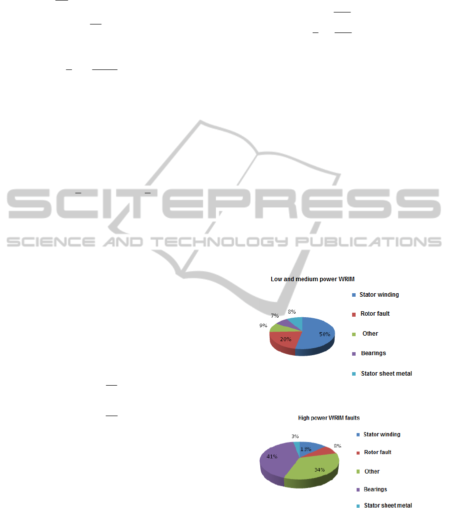
Figure 3: Low and medium power induction machines
faults (Razik, 2002; Chia-Chou et al., 2008).
Figure 4: High power induction machines faults (Razik,
2002; Chia-Chou et al, 2008).
Figure 3 and figure 4 present the faults
distribution carried out by a German company on
industrial system. The figure 3 show the faults of the
low and medium power machines (50 KW à 200
KW), and the figure 2 those of the high power
PRINCIPAL COMPONENTS ANALYSIS METHOD APPLICATION IN ELECTRICAL MACHINES DIAGNOSIS
169

machines (from 200 KW)
(Razik, 2002; Chia-Chou et
al., 2008)
.
Figure 3 shows that the most encountered faults
of the low and medium power on the induction
machines are the stator faults and the figure 4 shows
that the faults due to mechanical defects give the
highest percentages. The induction machines faults
can be classified into four categories (
Chia-Chou et
al., 2008
):
The stator faults can be found on the coils or the
breech. In most cases, the winding failure is caused
by the inter-turns faults. These last grow and cause
different faults between coils, between several
phases or between phase and earth point before the
deterioration of the machine (Sin et al., 2003). The
breech of electrical machines is built with insulated
thin steel sheets in order to minimize the eddy
currents for a greater operational efficiency. In the
case of the medium and great power machines, the
core is compressed before the steel sheets
emplacement to minimize the rolling sheets
vibrations and to maximize the thermal conduction.
The core problems are very little, only 1% compared
to winding problems (Negrea, 2006).
The rotor faults can be bar breaks, coils faults or
rotor eccentricities.
The bearings faults can be caused by a poor choice
of materials during the manufacturing steps, the
problems of rotation within the breech caused by
damaged, chipped or cracked bearing and can create
disturbance within the machines.
The other faults can be caused by the flange or the
shaft faults. The faults created by the machine flange
are generally caused during the manufacturing step.
Although the induction machines are robust, they
can be seats of different types of faults that can be
classified into two categories (Kliman et al., 1996):
• The hard and brutal faults modelised by an abrupt
inputs change or system parameters.
• The soft and arising faults due to gradual changes
of system parameters compared to their normal
values.
As previously mentioned, for the state survey of the
electrical machines, the PCA method was adopted.
3 PCA METHOD APPROACH
The PCA principle is based on simple linear algebra.
It can be used as exploring tool, analyzing data and
models design. The PCA method is based on a
transformation of the space representation of the
simulation data. The new space dimension is smaller
than that the original space dimension. It is classified
as without models method categories (Liu, 2006). It
can be considered as a full identification method of
physical systems (Marx et al., 2007; Ku et al., 1995;
Huang, 2001). The PCA allow to provide directly
the redundancy relations between the variables
without identifying the state representation matrix of
the system. This task is often difficult to achieve.
3.1 PCA Method Formulation
We note by x
i
(j) = [x
1
x
2
x
3
…x
m
] the measurements
vector « i » represents the measurement variables
that must be monitored and ranging from 1 to m and
« j » the number of the performed measurements for
each variable « m », ranging from 1 to N.
The measurements data matrix (X
d
€ R
N*m
) can
be written:
⎟
⎟
⎟
⎠
⎞
⎜
⎜
⎜
⎝
⎛
=
)(...)(
.........
)1(...)1(
1
1
NxNx
xx
X
m
m
d
(15)
This data matrix can be described with a possible
smallest set of new synthetic matrix, that is a
orthogonal linear projection of a subspace of m
dimension in a less dimension subspace l (l<m). The
method consists in identifying the PCA model and is
based on two steps (Li and Qin, 2001):
• Determination on the eigenvalues and the
eigenvectors of the covariance matrix R.
• Determination of the structure of the model, which
consists to calculate the components number « l » to
be retained in the PCA model.
3.2 Eigenvalues and Eigenvectors
Determination
Variables must be centered and reduced to make
data matrix independent of variables physical units.
Then, the new obtained normalized measures
matrix is:
]...[
1 m
XXX
=
(16)
And the covariance matrix R is given by:
T
XX
N
R
1
1
−
=
(17)
In decomposing R, (16) can be expressed as:
T
P
P
R
Λ
=
(18)
With
ICINCO 2011 - 8th International Conference on Informatics in Control, Automation and Robotics
170

m
TT
IPPPP ==
(19)
Λ
is diagonal matrix of the eigenvectors of R and
their eigenvalues are ordered in descending order
with respect to magnitude values (
)...
21 m
λ
λ
λ
≥≥≥ .
The eigenvectors matrix P is expressed as:
],...,,[
21 m
pppP =
(20)
i
p is the orthogonal eigenvectors corresponding to
i
λ
. Then, the principal components matrix is:
XP
T =
(21)
mN
T
*
ℜ∈
3.3 PCA Model Construction
To obtain PCA model, the components number “l”
to be retained must be determined. This step is very
important for PCA construction. For that, many rules
have been proposed by (Li and Qin, 2001). Most are
from sometimes subjective heuristics method or
criteria used in system identification in privileging
the data matrix approximation of the data matrix. In
this paper, "average eigenvalues" criterion is used.
The principle is based on the determination of the
variances of each component with the centered and
reduced variables. The number of variables l to be
retained to construct the PCA model is equal to the
number of components whose variance is greater
than unity.
By taking into account the number of
components to be retained and by partitioning the
principal components matrix T, the eigenvectors
matrix P and the eigenvalues matrix
Λ
(Valle et al.,
1999; Benaicha et al., 2010), the constructed PCA
model is given by:
[
]
)(** lmN
r
lN
p
TTT
−
=
(22)
[
]
)(** lmN
r
lN
p
PPP
−
=
(23)
⎥
⎥
⎥
⎦
⎤
⎢
⎢
⎢
⎣
⎡
Λ
Λ
=Λ
−− ))((
*
0
0
lmlm
ll
L
MOM
L
(24)
p
T
and
r
T is respectively the principal and residual
parts of T,
p
P
and
r
P is respectively the principal
and residual parts of P.
With this PCA model, the centered and reduced
matrix X can be written as:
T
rr
T
pp
TPTPX +=
(25)
In considering:
∑
=
==
l
i
T
ii
T
ppp
TPTPX
1
(26)
∑
+=
==
m
li
T
ii
T
rr
TPTPE
1
(27)
The centered and reduced matrix data is given by:
p
X
XE
=
+
(28)
p
X
is the principal estimated matrix and E the
residues matrix which represent information losses
due to the data matrix
X reduction. It represents the
difference between the exact and the approached
representations of
X. This matrix is associated with
the lowest eigenvalues
1
,...,
lm
λ
λ
+
. Therefore, in this
case, data compression preserves all the best the
information that it conveys. Under the application of
PCA at diagnosis, the number of components has a
significant impact on each step of faults detection
and localization procedure.
Nine state variables (m=9) have been chosen to
be monitored and 10000 measures (N=10000)
during 4s are considered. The WRIM faults are
introduced from the initial time (t=0s) to the final
time (t=4s) of the different simulations. The machine
is coupled to a mechanical load torque (10Nm) at
t=2s. The considered faults are respectively,
increases from 10% to 40% of the resistance value
of both the stator and rotor coils.
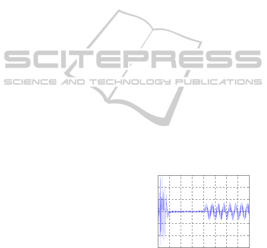
The following figures (Fig. 5 and Fig. 6)
represent the residues variation of the WRIM stator
current versus time and show the number
l impact in
the diagnosis approach:
Figure 5: Stator current residue for l = 5.
Figure 6 show that the chosen number of
components is too high then the residual space
dimension is reduced. Some faults are projected in
0 0.5 1 1.5 2 2.5 3 3.5 4
-1.5
-1
-0.5
0
0.5
1
1.5
Phase "A" stator current
Time [s]
PRINCIPAL COMPONENTS ANALYSIS METHOD APPLICATION IN ELECTRICAL MACHINES DIAGNOSIS
171

the principal space and the stator current residues
can not be detectable.
Figure 6: Stator current residue for l = 6.
However, with the figure 5, the number of
components is well chosen. Faults can be detected
and localized and the PCA model is well
reconstructed.
Generally, the detection approach in the case of
diagnosis based on analytical model is linked with
the residues generation step. From these residues
analysis, the decision making step must indicate if
faults exist are not. The residues generation
approach can be the state estimation approach or the
parameter estimation approach.
The residue indicates the information losses
given by the matrix dimension reduction of the state
variables matrix data to be monitored. Indeed, a
small residue means that the estimated value tends to
the exact value in healthy operation case.
In our case, the eigenvalues corresponding to the
number of the retained principal components
represent 93% of the total sum of eigenvalues. 0nly
7% of the total represent the residues subspace. One
can conclude that the PCA model has been well
constructed.
4 PCA METHOD APPLICATION
ON WRIM
The WRIM data simulation approaches with the
PCA method are given by the following figure:
Figure 7: Synoptic diagram of the different steps of the
data treatment.
The simulation approach is divided in four blocs:
• WRIM modeling: mathematical equations
calculation and simulation.
• Simulations results: graph showing the output
states of the system (healthy and faulted operation)
• Simulations data: simulation results acquisition as
matrix form.
• PCA: data treatment and system diagnosis.
4.1 Considered Faults
In normal operation, a resistance value variation
compared to its nominal value (in ambient
temperature, 25°C) is considered as faulted machine
due to machine overload or coils fault (Razik, 2002).
The resistance versus the temperature is
expressed as:
)1(
0
TRR
Δ
+
=
α
(29)
0
R is the resistance value at T
0
= 25°C,
α
the
temperature coefficient of the resistance and
T
Δ
the
temperature variation.
4.2 Simulation Results
The different simulation results have been
performed with respect to the simulation conditions
mentioned earlier.
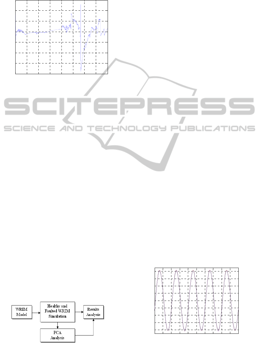
Figure 8 to figure 17 represent the real variations
without PCA method (Fig. 8 to Fig. 14) and the
residue variations with PCA application (Fig. 15 to
Fig. 17) of the faulted WRIM state variables in
considering stator faults.
With the WRIM state variables, other quantities
issued to their transformations have been calculated:
• quadrature axis and direct axis currents with Park
transformation,
•
α
axis and
β
axis currents with Concordia
transformation.
0 0.5 1 1.5 2 2.5 3 3.5 4
-8
-6
-4
-2
0
2
4
6
x 10
-7
Phase "A" stator current
Time [s ]
3.2 3.21 3.22 3.23 3.24 3.25 3.26 3.27 3.28 3.29 3.3
-8
-6
-4
-2
0
2
4
6
8
Stator phase "A" current [A]
Time [s ]
ICINCO 2011 - 8th International Conference on Informatics in Control, Automation and Robotics
172

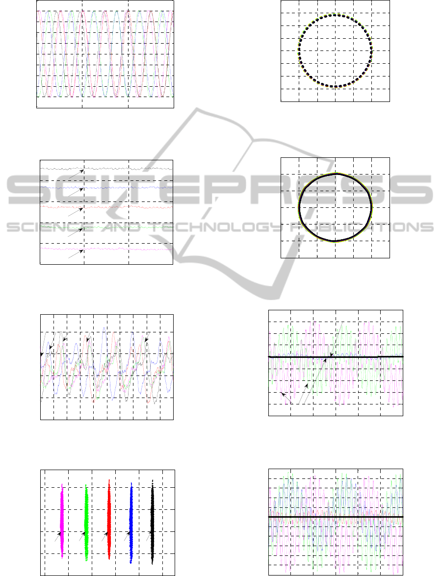
Figure 8: Real variations versus time of the stator current
of the healthy and faulted WRIM.
Figure 9: Real variations versus time of the rotor current
of the healthy and faulted WRIM.
Figure 10: Real variations versus time of the shaft
rotational speed of the healthy and faulted WRIM.
Figure 11: Real variations versus time of the
electromagnetic torque of the healthy and faulted WRIM.
Figure 12: Real variations of electromagnetic torque
versus the shaft rotational speed of the WRIM.
Figure 13: Real variations of
β
axis current versus the
phase
α
axis current of the stator phase.
Figure 14: Real variations of the quadrature axis current
versus the phase direct axis current of the stator phase.
Figure 15: Variations of the stator phase “A” current
residues versus time of the healthy and faulted WRIM.
2.5 3 3.5 4
-10
-8
-6
-4
-2
0
2
4
6
8
10
Rotor phase "a" current [A]
Time [s ]
2.5 3 3.5 4
287.5
288
288.5
289
289.5
290
Shaft rotational speed [rad/s]
Tim e [s ]
Healthy
10%
20%
30%
40%
2.8 2.82 2.84 2.86 2.88 2.9 2.92 2.94 2.96 2.98 3
10.3
10.35
10.4
10.45
10.5
Electromagnetic torque [Nm]
Tim e [s ]
40%
10%
20% 30%
Healthy
287.5 288 288.5 289 289.5 290
10.3
10.35
10.4
10.45
10.5
Electromagnetic torque [Nm]
Shaft rotational speed [rad/s]
40%
30%
20%
10%
Healthy
-15 -10 -5 0 5 10 15
-20
-15
-10
-5
0
5
10
15
20
Beta axis current [A]
Alpha axis current [A]
-15 -10 -5 0 5 10 15
-15
-10
-5
0
5
10
15
Quadrature axis current [A]
Direct axis current [A]
2.8 2.9 3 3.1 3.2 3.3 3.4
-1
-0.8
-0.6
-0.4
-0.2
0
0.2
0.4
0.6
0.8
Phase "A" stator current
Time [s ]
Healthy
Faulted
2.8 2.9 3 3.1 3.2 3.3 3.4
-1
-0.8
-0.6
-0.4
-0.2
0
0.2
0.4
0.6
0.8
1
Phase "a" rotor current
Time [s ]
PRINCIPAL COMPONENTS ANALYSIS METHOD APPLICATION IN ELECTRICAL MACHINES DIAGNOSIS
173

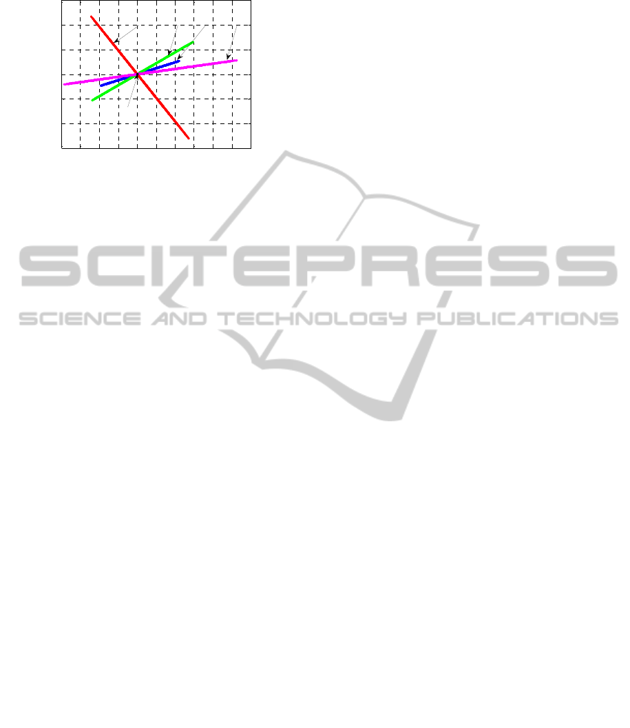
Figure 16: Variations of the rotor phase “a” current
residues versus time of the healthy and faulted WRIM.
Figure 17: Variations of electromagnetic torque residues
versus the shaft rotational speed residues of the WRIM.
4.3 Discussion
Several types of representations are used in the
signals processing domain, in particular for electrical
machines diagnosis. We can mention the temporal
representation (Fig. 8 to Fig.11, Fig. 15 and Fig. 17)
and the signal frequency analysis. Although they
have demonstrated their effectiveness, the state
variables representations between them also show
their advantages. They can be performed without
mathematical transformation (Fig. 12) and with
mathematical transformation (Fig. 13 and Fig. 14).
The latter representation type and the temporal
representation are confronted with the PCA method
application results (Fig. 15 to Fig. 17). Only the
simulation results with stator faults are presented
because the global behavior of the state variables in
both rotor and stator faults are almost similar.
For the temporal variations case, the rotor
currents (Fig. 9) and the shaft rotational speed (Fig.
10) are the variables which produce the most
information in presence of faults. The faults occur
on the rotor current frequency and the shaft
rotational speed magnitude.
Also, the electromagnetic torque variations
versus the shaft rotational speed clearly show the
WRIM operation zone in the presence of faults (Fig.
12). Contrary to this, the representations with
mathematical transformations (Fig. 13 and Fig. 14)
do not provide significant information due to the fact
that the stator currents remain almost unchanged in
the presence of faults (Fig. 8).
With PCA method application, all representation
types well show the differences between healthy and
faulted WRIM (Fig. 15 to Fig. 17). In the healthy
case, residues are zero. When faults appear, the
residue representations have an effective value with
an absolute value greater than zero.
In the figure 17, the healthy case is represented
by a point placed on the coordinate origins. Also,
one can show several right lines corresponding to
the faulted cases. This behavior is due to the
proportional characteristic of the considered faults.
PCA method proved so effective in electrical
machines faults detection. This requires a good
choice of the number of the principal components to
be retained so that information contained in residues
is relevant.
5 CONCLUSIONS
PCA method based on residues analysis has been
established and applied on WRIM diagnosis.
An accurate analytical model of the machine has
been proposed and simulated to performed the
healthy and faulted data for PCA approach need.
Several representations of nine state variables of
the machine have been analyzed. In the case of
temporal variation and without PCA, the rotor
current and the shaft rotational speed are the more
affected by the considered fault type. The
representations of the electromagnetic torque versus
the shaft rotational speed in both with and without
PCA approach show clearly the presence of faults.
Indeed, PCA method is interesting for all type of
representation compared to some other signal
processing types.
ACKNOWLEDGEMENTS
This research was supported by MADES/SCAC
Madagascar project. We are grateful for technical
and financial support.
REFERENCES
Wieczorek, M., Rosołowski, E., 2010. Modelling of
induction motor for simulation of internal faults,
Modern Electric Power Systems 2010, Wroclaw,
Poland MEPS'10 - paper P29.
Razik, H., 2002. Le contenu spectral du courant absorbé
par la machine asynchrone en cas de défaillance, un
état de l’art, La revue 3EI, n°29, pp. 48 - 52.
Chia-Chou, Y. & al., 2008. A Reconfigurable Motor for
Experimental Emulation of Stator Winding Interturn
and Broken Bar Faults in Polyphase Induction
Machines, IEEE transactions on energy conversion,
vol.23, n°4, pp. 1005-1014.
-0.4 -0.3 -0.2 -0.1 0 0.1 0.2 0.3 0.4 0.5 0.6
-0.4
-0.2
0
0.2
0.4
0.6
Electromagnetic torque
Shaft rotational speed
Healthy
40%10%20% 30%
ICINCO 2011 - 8th International Conference on Informatics in Control, Automation and Robotics
174

Sin, M. L., Soong, W. L., Ertugrul, N., 2003. Induction
machine on-line condition monitoring and fault
diagnosis – a survey, University of Adelaide.
Negrea, M. D., 2006. Electromagnetic flux monitoring for
detecting faults in electrical machines, PhD, Helsinki
University of Technology, Department of Electrical
and Communications Engineering, Laboratory of
Electromechanics, TKK Dissertations 51, Espoo
Finland.
Kliman, G. B., Premerlani, W. J., Koegl, R. A., Hoeweler
D., 1996. A new approach to on –line fault detection
in AC motors, San Diego, in Proc. IEEE Industry
Applications Society Annual Meeting Conference, CA,
pp. 687-693.
Liu, L., 2006. Robust fault detection and diagnosis for
permanent magnet synchronous motors, PhD
dissertation, College of Engineering, The Florida
State University, USA.
Marx, B., Mourot, G., Maquin, D., Ragot, J., 2007.
Validation et réconciliation de données. Approche
conventionnelle, difficultés et développements,
Workshop Interdisciplinaire sur la Sécurité Globale,
WISG’07, Troyes, France.
Ku, W., Storer, R. H., Georgakis, C., 1995. Disturbance
detection and isolation by dynamic principal
component analysis. Chemometrics and Intelligent
Laboratory Systems, 30, pp. 179–196.
Huang, B., 2001. Process identification based on last
principal component analysis, Journal of Process
Control, 11, pp.19–33.
Li, W., Qin, S. J., 2001. Consistent dynamic pca based on
errors-in-variables Subspace identification, Journal of
Process Control, 11(6), pp. 661–678.
Benaicha, A., Mourot, G., Guerfel, M., Benothman, K.,
Ragot, J., 2010. A new method for determining PCA
models for system diagnosis, 18th Mediterranean
Conference on Control & Automation Congress
Palace Hotel, Marrakech, Morocco June 23-25, pp.
862-867.
Valle, S., Weihua, L., Qin, S. J., 1999. Selection of the
number of principal components: The variance of the
reconstruction error criterion with a comparison to
other methods, Industrial and Engineering Chemistry
Research, vol. 38, pp. 4389-4401.
Harkat, M. F., Mourot, G., Ragot, J., 2005. An improved
PCA scheme for sensor FDI: Application to an air
quality monitoring network, Preprint submitted to
Elsevier Science.
PRINCIPAL COMPONENTS ANALYSIS METHOD APPLICATION IN ELECTRICAL MACHINES DIAGNOSIS
175