
REAL-TIME ELLIPSE FITTING, 3D SPHERICAL OBJECT
LOCALIZATION, AND TRACKING FOR THE ICUB SIMULATOR
Nicola Greggio
1,2
, Alexandre Bernardino
2
, Cecilia Laschi
1
, Paolo Dario
1
and Jos´e Santos-Victor
2
1
ARTS Lab - Scuola Superiore S.Anna, Polo S.Anna Valdera, Viale R. Piaggio 34, 56025 Pontedera, Italy
2
Instituto de Sistemas e Rob´otica, Instituto Superior T´ecnico, 1049-001 Lisboa, Portugal
Keywords:
Humanoid robotics, Machine vision, Pattern recognition, Least-square fitting, Algebraic distance.
Abstract:
This paper presents the implementation of real-time tracking algorithm for following and evaluating the 3D
position of a generic spatial object. The key issue of our approach is the development of a new algorithm
for pattern recognition in machine vision, the Least Constrained Square-Fitting of Ellipses (LCSE), which
improves the state of theart ellipse fitting procedures. It is a robust and direct method for the least-square fitting
of ellipses to scattered data. Although it has been ellipse-specifically developed, our algorithm demonstrates to
be well suitable for the real-time tracking any spherical object, and it presents also robustness against noise. In
this work we applied it to the RobotCub humanoid robotics platform simulator. We compared its performance
with the Hough Transform and with its original formulation, made by Fitzgibbon et Al. in 1999, in terms of
robustness (success/failure in the object detection) and fitting precision. We performed several tests to prove
the robustness of the algorithm within the overall system. Finally we present our results.
1 INTRODUCTION
The impressive advance of research and development
in robotics and autonomous systems over the past few
years has led to the development of robotic platforms
of increasing motor, perceptual, and cognitive capa-
bilities. These achievements are opening the way for
new application opportunities that will require these
systems to interact with other robots or nontechni-
cal users during extended periods of time. The final
goal is creating autonomous machines that learn how
to execute complex tasks and improve their perfor-
mance throughout their lifetime. Motivated by this
objective the RobotCub (ROBotic Open-Architecture
Technology for Cognition, Understanding and Behav-
ior) project has been developed (Sandini et al., 2007).
This is a research initiative dedicated to the realization
of embodied cognitive systems.
1.1 Related Work
The detection of circular objects is fundamental
in many applications, other than the developmental
RobotCub scenarios. An example is in the rescue em-
ployment of robotics platforms. Common situations
that employ rescue robots are mining accidents, ur-
ban disasters, hostage situations, and explosions. Cur-
rently, the research in rescue robotics is very fruitful
(Carpin et al., 2007). In addition, the NIST imple-
mented a simulator, USARSim (Urban Search And
Rescue Simulation) in order to develop rescue robots
(Wang et al., 2003). A clear and precise object recog-
nition is fundamental for such robots to find an acci-
dent victim as soon as possible with the highest pre-
cision as possible. Circular ad elliptical objects can
occur in body parts, such as head, and eyes. Vamossy
et Al. applied an ellipse detection algorithm to a res-
cue robot (Vamossy et al., 2003) in 2003, while, more
recently, Greggio et Al. used an ellipse detection al-
gorithm for recognizing the ball within the RoboCup
context (Greggio et al., 2009).
Other work in the robotics implementation of el-
lipse pattern recognition techniques has been per-
formed. Deniz et Al. used an ellipse detection al-
gorithm for face detection (Deniz et al., 2002). In
their work the authors focussed more on Human-
computer interaction. Moreover, Vincze et Al. used
a RANSAC-like method to find ellipses in real-world
examples (Vincze et al., 2000). They made exper-
iments to validate the capabilities of the approach
with in real contexts. Finally, Teutsch et Al. ap-
plied the ellipse recognition in industrial processes,
focussing on the real-time characteristics of their ap-
proach (Teutsch et al., 2006).
248
Greggio N., Bernardino A., Laschi C., Dario P. and Santos-Victor J..
REAL-TIME ELLIPSE FITTING, 3D SPHERICAL OBJECT LOCALIZATION, AND TRACKING FOR THE ICUB SIMULATOR.
DOI: 10.5220/0003543502480256
In Proceedings of the 8th International Conference on Informatics in Control, Automation and Robotics (ICINCO-2011), pages 248-256
ISBN: 978-989-8425-75-1
Copyright
c
2011 SCITEPRESS (Science and Technology Publications, Lda.)

1.2 Our Contribution
In this paper we implemented for the first time in a
real context our least-square fitting of ellipses tech-
nique (Greggio et al., 2010). We tested our new al-
gorithm, the B2AC (Fitzgibbon et al., 1999), and the
Hough transform (Leavers, 1992) under the same ex-
perimental conditions. We choose an actual task, i.e.
3D localization of a ball, and we compared these al-
gorithms’ performance in terms of overall localiza-
tion precision, and their robustness in terms of suc-
cess/failure detection of the object. We used the
simulation of a state of art robotics platform, the
RobotCub, in order to test it at best before doing this
with the real platform.
1.3 Outline
This paper is organized as follows. In sec. 2 we
will discuss the state of the art problem of the least-
square fitting of ellipses, the original algorithm and
its drawbacks with some solutions proposed in the re-
cent years. In sec. 3 we will propose our approach for
sidestepping the original numerical instability prob-
lem. Then, in sec. 4 we will describe the RobotCub
robotics platform, in terms of its mechanics and the
simulator we used. Furthermore, in section 5 we will
briefly explore our vision algorithms. In sec. 6 we
will describe our experimental set-up. In sec. 7 we
will discuss our results. Finally, in sec. 8 we will
conclude our work and explain our projects as future
research.
2 LEAST SQUARE FITTING OF
ELLIPSES
2.1 The State of the Art
Two main approaches can be considered for circle de-
tection. The first one is to use the Hough Transform
(Yuen et al., 1989). Since spatial perspective alters
the perceived objects, there is the need of calibrating
the camera(s). Then, a pattern recognition algorithm,
such as a simple color detection, can be applied and
subsequently the Hough circle transform can be ap-
plied in order to estimate all the ball’s features.
However, this approach can be complex to be im-
plemented, and even elevate resource consumption.
First, it requires the camera calibration. Moreover,
it can be argued that using a Hough Transform, for
instance, by augmenting the image’s resolution the
computational burden increases as well. Finally, the
Hugh transform needs to be set well, in terms of the
accumulator threshold at the center detection stage
parameter.
The second one is to use ellipse specific pat-
tern recognition algorithms, such as (Maini, 2006),
(Fitzgibbon et al., 1999). By processing a ball think-
ing of it as it were an ellipse, we overcome the distor-
tion problems. Circles in man-made scenes are almost
always distorted when projected onto the camera im-
age plane, therefore generating ellipses.
Some techniques based on Least Square (LS)
came out in recent years (Fitzgibbon et al., 1999),
(Gander et al., 1994). The principal reason is because
of its computational costs. There are two main kinds
of LS techniques: Those based on the minimization
of the algebraic (Algebraic Distance Least Square,
ADLS) and geometric distance (Geometric Distance
Least Square, GDLS)between the data points and the
ideal curve and those based on the minimization of
the geometric distance ADLSs suffer of high curva-
ture bias (Kanatani, 1994) with the the non-invariance
to Euclidean transformation (Zhang, 1997). However,
GDLSs suffer of being dependent of iterative algo-
rithms (Rosin and West, 1995) as do cluster/voting
(CV) techniques, therefore making them not suitable
for real-time applications (Fitzgibbon et al., 1999).
This is a notable drawback, because iterative algo-
rithms do not have a fixed computational time. Nev-
ertheless, algebraic fitting algorithms may guarantee
a direct one-step convergence. We will focus on this
way, starting from the work of Fitgibbon et Al., called
B2AC, which will be described in the next section
(Fitzgibbon et al., 1999).
2.2 The Original Algorithm
A central conic can be expressed by a second order
equation in its implicit form, as follows in the eq. (eq.
1):
F(x,y) = ax
2
+ bxy+ cy
2
+ dx+ ey+ f = 0 (1)
This can also be expressed in the vectorial form:
F
a
(x) = x· a =0 (2)
where a =[a, b,c, d,e, f]
T
is the vector of the equation
coefficients, and x =[x
2
,xy,y
2
,x,y,1] is the vector of
the points’ coordinates, both relative to the conic sec-
tion.
Assuming F(a, p
i
) as the algebraic distance from
the point p
i
= (x
i
,y
i
) to the conic expressed by (eq. 2)
the following non-linear minimization problem has to
be solved (DeSouza and Kak, 2002):
min
a
(
N
∑
i=1
F(a,p
i
)) = min
a
(
N
∑
i=1
F(a· p
i
)
2
) (3)
REAL-TIME ELLIPSE FITTING, 3D SPHERICAL OBJECT LOCALIZATION, AND TRACKING FOR THE ICUB
SIMULATOR
249

In (Fitzgibbon et al., 1999) Fitzgibbon et Al. demon-
strated that solving the problem with the following
constraints gives rise to a unique exact solution:
minkD· ak
2
a
T
· C· a = 1
(4)
where
D =
x
2
1
x
1
y
1
y
2
1
x
1
y
1
1
.
.
.
.
.
.
.
.
.
.
.
.
.
.
.
.
.
.
x
2
N
x
N
y
N
y
2
N
x
N
y
N
1
(5)
and C is a 6 × 6 symmetric matrix where C
(1,3)
= 2,
C
(2,2)
= −1, and C
(3,1)
= 2.
Now, by using the Lagrange mulltiplier λ and dif-
ferentiating we obtain:
2D
T
Da− 2λCa = 0
a
T
· C· a = 1
(6)
or in the form:
Sa = λCa
a
T
· C· a = 1
S = D
T
D
(7)
Finally, Fitzgibbon and colleagues demonstrated
that ˜a
i
= µ
i
u
i
is a unique solution of the system equa-
tions in (eq. 4) (Fitzgibbon et al., 1999), where:
µ
i
=
s
1
u
T
i
Cu
i
=
s
λ
i
u
T
i
Su
i
(8)
Therefore, the correspondent affine anti-
transformation (Maini, 2005) needs to be performed
after having found the optimal solution ˜a
6
.
Some improvements to the original method
(Fitzgibbon et al., 1999) have been made within the
last years. One deserves particular noticing. In
(Maini, 2005) it has been proposed to compute the
following affine transformation to the input points
before applying the Fitzgibbon’s et Al. algorihm
(Fitzgibbon et al., 1999) :
˜x =
x− x
m
s
x
− 1 ˜y =
y− y
m
s
y
− 1 (9)
where x
m
= min
N
i=1
x
i
and y
m
= min
N
i=1
y
i
and:
s
x
=
max
N
i=1
x
i
− min
N
i=1
x
i
2
s
y
=
max
N
i=1
y
i
− min
N
i=1
y
i
2
(10)
2.3 Drawbacks and Our Improvement
In 2006 Maini criticized the ill-conditioning of the
scatter matrix S = D
T
D (eq. 7) and proposed an affine
transformation for solving it by recentering the el-
lipse points within a square with side length equals
to 2 (Maini, 2006). Moreover, in (Maini, 2006) it has
been reported that the algorithm in (Fitzgibbon et al.,
1999) has a specific source of errors not mentioned in
the paper, and that this causes numerical instabilities,
giving rise to the fact that the closer the data points are
to the ellipse (i.e. the less noise is present), the more
difficult is to locate a unique solution. This results
in the impossibility of having a solution (i.e. a pre-
cise and unique ellipse curve equation) when the data
points lie exactly on, or too close to, the ideal ellipse
curve. In (Maini, 2005), and (Maini, 2006), a resam-
pling procedure has been proposed, that perturbs the
data points with gaussian noise in the case of they are
too close to the ellipse. However, this requires an ex-
cessive computational burden. In fact, he claims that
the procedure must be applied an adequate number
of times M in order to make the algorithm effectively
robust. This makes this approach it not suitable for
real-time applications.
In this work we propose the application of a new
pattern recognition algorithm for the least square of
ellipses we presented in (Greggio et al., 2010) that
overcomes the numerical instability of the original
formulation (Fitzgibbon et al., 1999). Our solution
takes advantage of the improvements given in (Maini,
2006) in terms of the input affine transformation (eq.
9, 10), while using a less expensive computational
perturbing function.
3 LCSE: LEAST CONSTRAINED
SQUARE-FITTING
OF ELLIPSES
3.1 Instability of the Exact Ellipse
Solution
In this section we propose a technique that overcomes
the previous problems. We decided to perturb the
ellipse’s polar transformation by adding a periodic
symmetric function. We apply the data perturbation
only if the case of not stable numerical solution, as
in (Maini, 2006). However, due to our low compu-
tational burden, it does not affect the total computa-
tion sensibly, and can therefore be used any time is
required. The scheme is illustrated in Fig. 1.
The procedure is then described as follows:
• (a) Application of the affine transformation
(Maini, 2006).
• (b) Transformation from the cartesian coordinates
ICINCO 2011 - 8th International Conference on Informatics in Control, Automation and Robotics
250

Figure 1: The RobotCub’s Head. On the left image the head
without the cover is shown, while in the right image the
cover is shown.
Figure 2: the original ellipse after the recentering procedure
(top-left), that represented in polar coordinates (middle), the
polar transformed ellipse with the sinusoidal perturbation
(bottom), and the resultant perturbed ellipse (top-right).
(x,y) to the polar ones (ρ,θ). The point i results:
ρ
i
=
q
x
2
i
+ y
2
i
θ
i
= arctan(
y
i
x
i
); with : x
i
≥ 0, y
i
≥ 0
θ
i
=
π
2
− arctan(
x
i
y
i
); with : x
i
≤ 0, y
i
≥ 0
θ
i
= π + arctan(
y
i
x
i
); with : x
i
≤ 0, y
i
≤ 0
θ
i
=
3π
2
− arctan(
x
i
y
i
); with : x
i
≥ 0, y
i
≤ 0
(11)
Our aim is to move the points around their initial
position, but maintaining the ellipse average over the
whole polar representation period (2π) within its po-
lar representation. Any symmetric periodic function
with period taken as integer multiplier of 1 added to
the original scattered data leaves the ellipse polar av-
erage unaltered. Therefore, we choose the sinusoidal
function, being continuous, easy to be implemented,
with zero average and infinitely derivable.
• (c) We choose the amplitude equals to A = 0.001
and the frequency equals to f = 1000Hz. The
point i obeys to:
ˆ
ρ
i
= ρ
i
+ A· sin(2π fθ
i
); (12)
• (d) When the ellipse is remapped in cartesian co-
ordinates, its results equally slightly perturbed in-
side and outside its ideal curve, which is the curve
that best interpolates these data. It results, for the
point i:
ˆx
i
=
ˆ
ρ
i
· cos(θ
i
);
ˆy
i
=
ˆ
ρ
i
· sin(θ
i
);
(13)
• (e) Now the ellipse is ready to be fitted by build-
ing the design matrix (eq. 5), and by solving the
eigenvalues problem (eq. 7).
• (f) Finally, the affine denormalization transforma-
tion of the point (a) has to be applied.
Fig. 2 shows the original ellipse after the recenter-
ing procedure (top-left), that represented in polar co-
ordinates (middle), the polar transformed ellipse with
the sinusoidal perturbation (bottom), and the resultant
perturbed ellipse (top-right).
3.2 Computational Burden Analysis
Now we analyze the computational complexity of the
algorithm proposed in (Maini, 2006), and our tech-
nique. Low computational complexity means higher
frame rates in real-time applications, and therefore
faster control loops. This results essential in many
actual applications (Vincze, 2001) (Kwolek, 2004)
(Nelson and Khosla, 1994). Our new approach is able
to eliminate the numerical instability that affects the
original algorithm (Fitzgibbon et al., 1999) as (Maini,
2006) does, but greatly faster. We consider N being
the number of points composing the ellipse scattered
data.
Now we will describe: (a.) the resampling pro-
cedure proposed in (Maini, 2006), (b.) our new ap-
proach, and (c.) the final comparison between these
two algorithms.
→ a. Resampling procedure: The complete pro-
cedure has been explained in (Maini, 2005). For each
point a gaussian noise component is added. There-
fore, this operation goes with O(N). Therefore the
sequence of operations relative to eq. 7 - 10, has to be
performed. This process goes with O(6N) + O(42N),
repeated for M times. Thus, the resultant complexity
is O(49MN). Finally, an averaging procedure through
all the ellipse data has to be performed, which makes
the overall process going with O(MN)+ O(49MN) =
O(50MN).
→ b. Add sinusoidal perturbation: This adds the
sinusoidal perturbation to the ellipse data after having
been transformed into polar coordinates (originally,
REAL-TIME ELLIPSE FITTING, 3D SPHERICAL OBJECT LOCALIZATION, AND TRACKING FOR THE ICUB
SIMULATOR
251

they are expressed in cartesian representation). Thus
there are three operations to be performed: the first
one is the transformation of all the data points from
cartesian to polar representation. This takes O(2N).
After that, the addition of the sinusoidal perturba-
tion takes O(N) operations. Then, the polar coordi-
nates are remapped into cartesian ones, taking O(2N).
Therefore, the whole operation goes with O(5N).
→ c. Computational comparison. In (Maini,
2006) it has been suggested 50 ≤ M ≤ 200. More-
over, it has been reported that EDFE performed better
performances than B2AC for M ≥ 200. However, this
costs an enormous computational burden. Even if M
were equal to 50, our procedure is 500 times faster
than (Maini, 2006). In fact, by comparing the latter
algorithm versus our procedure, it is possible to see
that our procedure is faster of O(50MN)/O(5N) ⇒
10M = 10· 50 = 500 times.
4 THE ICUB ROBOTIC
PLATFORM
The robot is composed of 53 degrees of freedom
(DOFs). Most of them are directly actuated, such as
the shoulders, others are under-actuated, such as the
hands.
In vision, the robotic head design plays an impor-
tant role. Both eyes can tilt (i.e. to move simultane-
ously up and down), pan (i.e. to move simultaneously
left and right), and verge (i.e. to converge or diverge,
with respect to the vision axes). The pan movement
is driven by a belt system, with the motor behind the
eye ball.
An exhaustive explanation about a kinematic and
a dynamic analysis for the upper body structure can
be found in (Nava et al., 2008).
4.1 The ODE iCub Simulation
On the one side, the simulator information is not ex-
haustive, but it is a good approximation for the soft-
ware debugging before using it on the real robot. On
the other side, our algorithm claims to overcome the
original Fitzgibbon’s approach drawback of failing in
detecting the ellipse when the curve lies on the ideal
curve (i.e. is case of noise absence.) (Maini, 2006).
It is clear that image segmentation in the real robot
will never, or very seldom, produce perfect ellipses
after image segmentation, due to all the imperfection
within the real word (light gradients, light contrasts,
color gradients, not regular object shapes, etc), there-
fore testing this ellipse pattern recognition algorithm
to the real robot will not produce comprehensive re-
sults. Contrariwise, the simulator does not present
these artifacts, or at least it limits them.
Tikhanoff et al. developed a completely open
source simulator for the iCub (Tikhanoff et al., 2008),
based entirely on the ODE (Open Dynamic Engine).
We use this simulator in order to test our algorithms.
Fig. 4 shows a print screen of the simulator.
5 SEC::AI034-CUB: THE ROBOT
CONTROLLING TOOL
5.1 The Vision Module
The vision module receives the images from the two
cameras mounted on the iCub head. In order to detect
the ball, and all its features, we implemented a simple
but efficient image processing algorithm. We identify
the ball by means of a color filter.
(a) The left camera output. (b) The object recognized within the
left camera.
Figure 3: The input image, as seen by the robot within the
simulator with the egocentric view (a) and the same image
with the superimposition of an ellipse, drawn by using the
characteristic parameters obtained by computing the LCSE
(b).
For the identification of the blob corresponding to
the ball, we use a connected components labeling al-
gorithm. We assume the largest blob is the ball, so we
look for the blob with the largest area. Subsequently,
we proceeded by applying our LS technique (Greggio
et al., 2010) to the found blob, in order to detect all
the parameters of the curve that describes the bound-
ary of the blob. In Fig. 3(a) the input to the left camera
is presented, i.e. the experimental scenario, while in
Fig. 3(b) output of the algorithm is presented.
5.2 The Motor Control Module
In addition, we implemented a tracking algorithm in
a closed loop. The information received from the vi-
sion module are then processed sent to the motors
ICINCO 2011 - 8th International Conference on Informatics in Control, Automation and Robotics
252
of the iCub’s head by means of a velocity control
scheme. that directly commands the head of the robot,
Then, using the forward robot’s kinematics and the
encoders’ information we are able to reconstruct the
target object’s center of gravity (COG) spatial posi-
tion.
1
. In Fig. 4 a screenshot is depicted, that shows
the testing scenario.
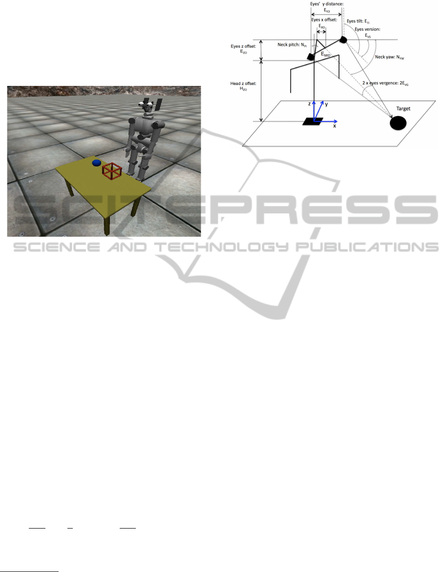
Figure 4: A screenshot depicting the simulated robot in the
3D surrounding environment. Our program uses the en-
coders information to triangulate the position of the centroid
of the object within the simulated space.
5.3 The Kinematics Module
Then, the Denavit-Hartemberg convention for the ob-
ject’s COG coordinates is analyzed. Fig. 5 illustrates
the schematization of the iCub’s neck-head-eyes sys-
tem. Then, tab. 1 contains the relative body kinemat-
ics lenghts, and tab. 2 shows the parameters of the
D-H symbols notation.
Here, the angles represent:
• θ
∗
1
: Neck pitch - positive up
• θ
∗
2
: Neck yaw - positive left
• θ
∗
3
: Eyes tilt - positive up
• θ
∗
4
: Eyes version - positive left
Then, d
0
represents the target’s COG distance
from the eyes’ middle axis point E
MID
(see Fig. 5).
This is evaluated with a simple geometrical relation-
ship, as follows:
d
0
=
E
YD
2
tan
π
2
− E
VG
=
E
YD
2
tan
−1
(E
VG
)
(14)
The target’s COG coordinates (x
COG
,y
COG
,z
COG
) are
evaluated as follows:
1
The reference system is centered on the floor plane, at
the center of the pole that sustains the robot. The x axis
evolves along the front of the robot, the y axis runs along
the left of the robot, and the z axis evolves along its height.
Figure 5: Schematization of the iCub’s kinematics. This is
not all the kinematics, of course. We focussed on the head
and neck’s joints.
x
COG
y
COG
z
COG
1
=
h
T
5
0
i
x
5
y
5
z
5
1
(15)
with:
T
5
0
=
cosθ
∗
1
cosθ
∗
2
cosθ
∗
3
cosθ
∗
4
+ −sinθ
∗
4
cosθ
∗
1
cosθ
∗
2
cosθ
∗
3
+
−cosθ
∗
1
sinθ
∗
2
sinθ
∗
4
−cosθ
∗
1
sinθ
∗
2
cosθ
∗
4
sinθ
∗
2
cosθ
∗
3
cosθ
∗
4
+ sinθ
∗
2
sinθ
∗
4
cosθ
∗
3
+
cosθ
∗
2
sinθ
∗
4
cosθ
∗
2
cosθ
∗
4
sinθ
∗
1
cosθ
∗
2
cosθ
∗
3
cosθ
∗
4
+ −sinθ
∗
1
sinθ
∗
4
cosθ
∗
2
cosθ
∗
3
+
−sinθ
∗
1
sinθ
∗
2
sinθ
∗
4
−sinθ
∗
1
sinθ
∗
2
cosθ
∗
4
0 0
−sinθ
∗
3
cosθ
∗
1
cosθ
∗
2
d
0
cosθ
∗
1
cosθ
∗
2
cosθ
∗
3
cosθ
∗
4
+
−d
0
sinθ
∗
4
cosθ
∗
1
sinθ
∗
2
+
l
L3
cosθ
∗
1
cosθ
∗
2
−sinθ
∗
2
sinθ
∗
3
−d
0
cosθ
∗
3
cosθ
∗
4
sinθ
∗
2
+
d
0
cosθ
∗
2
sinθ
∗
4
l
L3
sinθ
∗
2
−sinθ
∗
1
sinθ
∗
3
cosθ
∗
2
+ d
0
cosθ
∗
2
cosθ
∗
3
cosθ
∗
4
sinθ
∗
1
+
cosθ
∗
1
cosθ
∗
3
−d
0
sinθ
∗
1
sinθ
∗
2
sinθ
∗
4
l
L3
sinθ
∗
1
cosθ
∗
2
+
h
L1
cosθ
∗
1
+ h
L1
0 1
(16)
6 EXPERIMENTS
We performed three types of experiments:
a. The robot localizes a blue cylinder (obtained as
a section of the ball used in the experiment (b)),
and having a negligible height) in front of it; the
cylinder goes away along the x-axis direction at
each trial;
REAL-TIME ELLIPSE FITTING, 3D SPHERICAL OBJECT LOCALIZATION, AND TRACKING FOR THE ICUB
SIMULATOR
253

Table 1: Body kinematics lenghts.
Lenght
Symbol Meaning
[SMU]
0.35 E
YD
Eyes y distance: Related to the y axis, it represents the distance between the eyes along their axis
0.36 E
XO
Eyes x offset: Related to the x axis, it represents the distance between the neck pitch axis and the eyes axis
3.50 E
ZO
Eyes z offset: Related to the z axis, it represents the distance between the neck yaw axis and the eyes axes
3.01 H
ZO
Head z offset: Related to the z axis, it represents the distance between the origin of the reference system and
the neck pitch joint
b. The robot has to evaluate the ball’s radius while
an occlusion hides the object;
c. The robot has to localize a blue ball in front of it.
Table 2: Body kinematics Denavit-Hartenberg parameters.
Link a
i
α
i
d
i
θ
i
L
1
0 π/2 h
L1
0
L
2
0 -π/2 0 θ
∗
1
L
3
l
L3
π/2 h
L3
θ
∗
2
L
4
0 -π/2 0 θ
∗
3
L
5
d
0
0 0 θ
∗
4
Localization is intended in terms of 3D cartesian
coordinates. At each trial the Hough transform, the
B2AC, and the LCSE algorithms are used in order to
evaluate the ball’s center of mass (COM) within the
2D camera images. Therefore this information is tri-
angulated with the encoders’ values in order to deter-
mine the ball spatial position.
Since there is a prospective error, introduced by
the spatial perspective, the ball is not seen as a 2D cir-
cle by the two camera, hence distorted, bringing about
to an artifact during these scenarios experiments that
is not due to the goodness of the three tested algo-
rithms. In order to reduce this effect we tried to iso-
late the perspective error by performing the experi-
ment (a). For each scenario we performed at least 30
trials. The robot stands up and remains in the same
position.
We tested both the precision in localization and
the percentage of success/failure in detection.
7 RESULTS AND DISCUSSION
In the scenario a and b the error between the real and
the evaluated cylinder’s and ball’s position is deter-
mined, while in the scenario c the error between the
real and evaluated ball’s radius is calculated.
7.1 Error Propagation Evaluation
We evaluated the error propagation for the position
detection as follows. All of the terms are measured in
simulator measure unit (SMU). The err
pixel
is the ab-
solute error relative to the value of one square pixel.
In order to evaluate it we referred to the known ball’s
radius. By knowing it (as a fixed value, i.e. 0.17
SMU) and by evaluating it at each measure we can es-
timate the value of a square pixel in SMU (this is the
image resolution at the object distance) as the ratio
between the known radius and the one estimated with
each of the three algorithms considered (i.e. Hough
transform, B2AC, and LCSE).
The errors of the encoders can be considered neg-
ligible within the simulator. Since there is no docu-
mentation on the encoders’ resolution within the sim-
ulator, we considered the accuracy of their informa-
tion approximated to their last digit, which is the
forth one (therefore negligible). Finally the errors due
robot’s lengths need to be considered. Again, there
is no information about the error the lengths of the
robot’s parts have been expressed with. Therefore, in
order to fix their accuracy we analyzed the simula-
tor’s source code. So far, we found that the lengths of
the robot’s parts were expressed with the second digit
of approximation. Hence, we approximated them as
0.01 SMU.
7.2 Scenarios’ Evaluation
As a first result, Fig. 6(a) shows the results of the sce-
nario a. With exception for the quadratic error within
the range [2.15 − 2.35], the Hough Transform (HT)
gives rise to the highest error. Both the ellipse fitting
algorithms cause lower error. Specifically, the B2AC
algorithm is the most precise in terms of quadratic er-
ror, within the ranges [1.2− 1.9], and [2.7− 3.4]. The
LCSE seems to be not the lowest error prone, but it
has a very regular characteristic as a function of the
distance.
The experiment of the scenario b shows a great
linearity between the occlusion of the ball and the er-
ror on its radius evaluation. Fig. 6(b) illustrates the
results of this experiment. Here, the HT gets bet-
ter results within the range [5 % - 20 %] of occlu-
sion. The characteristic is quite linear for all the tech-
niques adopted, with the exception of the cited range,
in terms of a slight decrease from the linear ideal line
ICINCO 2011 - 8th International Conference on Informatics in Control, Automation and Robotics
254
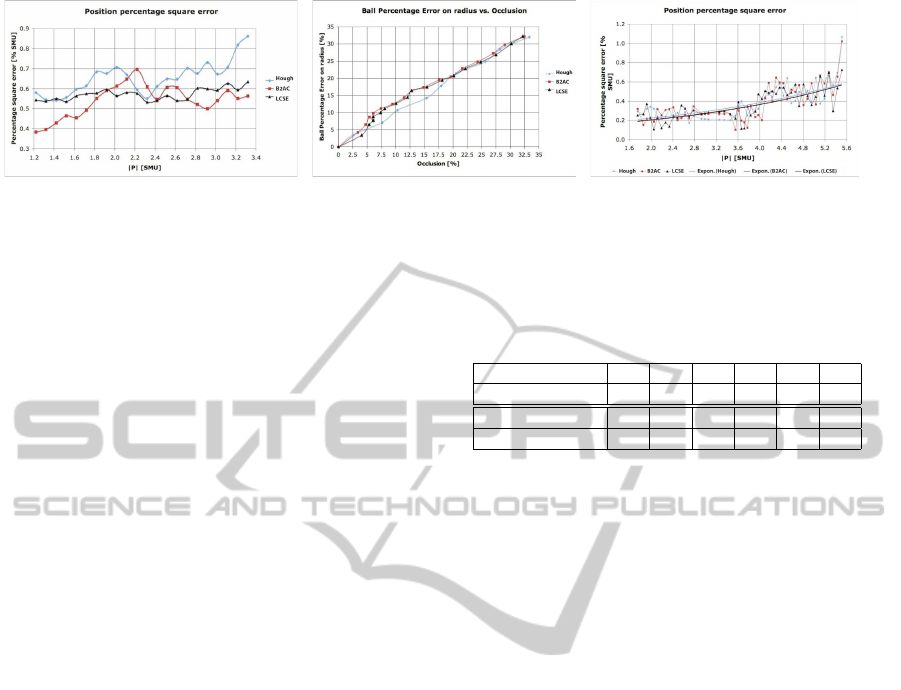
(a) (b) (c)
Figure 6: Cylinder’s position error as function of the distance while considering the perspective effect negligible (a), ball
Percentage Error on radius, in % of the radius value (b), and percentage square error, measured in % of the simulator measure
unit (c).
for the HT and a slight increment for both ellipse de-
tection approaches. The two ellipse recognition tech-
niques are more sensitive than the HT to the spatial
perspective.
Finally, the scenario c is discussed. The ellipse
detection approaches give rise to a bigger spatial per-
spective error than the HT within the whole tracking
system, even though the thy also bring about to a big-
ger spatial perspective error than the HT. In 6(c) this
is showed. We did not filter the results, in order to
keep them as natural as possible. Therefore, we in-
serted three trend lines (one for each technique, each
of them with exponential characteristic) in order to
evidence the most fruiting approach. The B2AC’s and
the LCSE’s trend lines appear superimposed, so that
it is not possible distinguishing them from each other.
The HT’s trend line is the most error prone for balls’
spatial position detection in image processing.
7.3 Some Aspects of the Hough
Transform
It is worth mentioning that the HT depends on some
parameters in order to work correctly. Particularly, we
refer to the accumulator threshold at the center de-
tection stage (ATCDS). The smaller its value is, the
more false circles may be detected, but the higher it is,
the less circles may be detected. The first case means
that other curvatures, e.g. artifacts on the ball’s bor-
der caused for instance by inaccuracies of the color
filtering, may be detected as additional objects. How-
ever, the second case can cause the opposite problem.
In our experiments there was only one circular object
within the image, the ball, but setting ATCDS too high
resulted in not detecting it. Therefore, we looked for
the biggest value able to perform all the experiments,
finding ATCDS = 2. In tab. 3 there are some ATCDS
values: Each one represents the maximum value able
to perform the experiments at some fixed occlusion
and distance values.
However, both B2AC and LCSE algorithms do
Table 3: Maximum value for the accumulator threshold for
getting stability in our experiments.
ATCDS 3 2.6 2.3 2.1 2 2
Occlusion [%] 5 10 15 20 25 30
ATCDS 3.4 3 2.6 2.4 2.1 2
Distance [SMU] 1.2 1.6 2 2.4 2.8 3.2
not present a similar drawback, permitting them to
be used in any situation without any previous setting.
This can be considered a great advantage, since they
do not require any a priori information of the scene to
be analyzed. This is twofold, because allows not only
to build a robust and scene− independent technique,
but also it fits with the concept of cognitive robotics
perfectly.
8 CONCLUSIONS
In this work we presented the first implementation of
the LCSE ellipse square fitting algorithm, and we ap-
plied it to a humanoid robotics platform. Moreover,
we implemented a real-time tracking algorithm to lo-
calize an object with the Robot’s stereo vision, and
subsequently we used it to determine the 3D position
of the object’s centroid in the environment. We com-
pared the Hough Transform, the B2AC, and the LCSE
performances in terms of localization precision and
failure in detection in presence of induced artifacts
(such as the ball occlusion by another object) and as
function of the distance of the target. We found that
the B2AC and LCSE give rise to overall more pre-
cise results than the Hough Transform. In the near fu-
ture we plan to apply our techniques to the real iCub
robotics platform, in order to compare and validate
our results with the real robot.
ACKNOWLEDGEMENTS
We thank Dr. Andrea Cini for his contribution in writ-
REAL-TIME ELLIPSE FITTING, 3D SPHERICAL OBJECT LOCALIZATION, AND TRACKING FOR THE ICUB
SIMULATOR
255

ing the DH matrix for the robot forward kinematics.
This work was supported by the European Com-
mission, Project IST-004370 RobotCub and FP7-
231640 Handle, and by the Portuguese Government -
Fundac¸˜ao para a Ciˆencia e Tecnologia (ISR/IST
pluriannual funding) through the PIDDAC program
funds and through project BIO-LOOK, PTDC / EEA-
ACR / 71032 / 2006.
REFERENCES
Carpin, S., Lewis, M., Wang, J., Balarkirsky, S., and Scrap-
per, C. (2007). Usarsim: a robot simulator for research
and education. In IEEE International Conference on
Robotics and Automation.
Deniz, O., Castrillon, M., Lorenzo, J., Guerra, C., Hernan-
dez, D., and Hernandez, M. (2002). Casimiro: A robot
head for human-computer interaction. Robot and Hu-
man Interactive Communication. Proceedings. 11th
IEEE International Workshop on, (ISBN: 0-7803-
7545-9):319– 324.
DeSouza, G. N. and Kak, A. C. (2002). Vision for mobile
robot navigation: A survey. IEEE Transaction PAMI,
24:237–267.
Fitzgibbon, A., Pilu, M., and Fisher, R. (1999). Direct least
square fitting of ellipses. IEEE Trans. PAMI, 21:476–
480.
Gander, W., Golub, G., and Strebel, R. (1994). Fitting of
circles and ellipses least squares solution. Technical
report tr-217, Institut f¨ur Wissenschaftliches Rechen,
ETH, Zurich, Switzerland.
Greggio, N., Bernardino, A., Laschi, C., Santos-Victor,
J., and Dario, P. (2010). An algorithm for the least
square-fitting of ellipses. IEEE 22th International
Conference on Tools with Artificial Intelligence (IC-
TAI 2010), Arras, France.
Greggio, N., Silvestri, G., Menegatti, E., and Pagello, E.
(2009). Simulation of small humanoid robots for soc-
cer domain. Journal of The Franklin Institute - Engi-
neering and Applied Mathematics, 346(5):500–519.
Kanatani, K. (1994). Statistical bias of conic fitting and
renormalization. IEEE Trans. Patt. Anal. Mach. In-
tell., 16:320–326.
Kwolek, B. (2004). Real-time head tracker using color,
stereovision and ellipse fitting in a particle filter. IN-
FORMATICA, 15(2):219–230.
Leavers, V. F. (1992). Shape detection in computer vision
using the hough transform. Springer-Verlag.
Maini, E. S. (2005). Robust ellipse-specific fitting for real-
time machine vision. BVAI, pages 318–327.
Maini, E. S. (2006). Enhanced direct least square fitting of
ellipses. IJPRAI, 20(6):939–954.
Nava, N., Tikhanoff, V., Metta, G., and Sandini, G. (2008).
Kinematic and dynamic simulations for the design of
robocub upper-body structure. ESDA.
Nelson, B. J. and Khosla, P. K. (1994). The resolvability el-
lipsoid for visual servoing. Proc. of the 1994 Conf. on
Computer Vision and Pattern Recognition (CVPR94).
Rosin, P. L. and West, G. A. (1995). Non parametric
segmentation of curves into various representations.
IEEE Trans. Patt. Anal. Mach. Intell., 17:140–153.
Sandini, G., Metta, G., and Vernon, D. (2007). The icub
cognitive humanoid robot: An open-system research
platform for enactive cognition. 50 Years of AI, M.
Lungarella et al. (Eds.), Festschrift, LNAI 4850, pages
359–370.
Teutsch, C., Berndt, D., Trostmann, E., and Weber, M.
(2006). Real-time detection of elliptic shapes for auto-
mated object. Machine Vision Applications in Indus-
trial Inspection XIV. Edited by Meriaudeau, Fabrice;
Niel, Kurt S. Proceedings of the SPIE, 6070:171–179.
Tikhanoff, V., Fitzpatrick, P., Nori, F., Natale, L., Metta,
G., and Cangelosi, A. (2008). The icub humanoid
robot simulator. International Conference on Intel-
ligent RObots and Systems IROS, Nice, France.
Vamossy, Z., Moolnar, A., Hirschberg, P., Toth, A., and
Mathe, B. (2003). Mobile robot navigation projects
at bmf nik. International Conference in Memoriam
John von Neumann.
Vincze, M. (2001). Robust tracking of ellipses at frame rate.
Pattern Recognition, 34:487–498.
Vincze, M., Ayromlou, M., and Zillich, M. (2000). Fast
tracking of ellipses using edge-projected integration
of cues. Pattern Recognition. Proceedings. 15th Inter-
national Conference on, 4(ISBN: 0-7695-0750-6):72–
75.
Wang, J., Lewis, M., and Gennari, J. (2003). Usar: A game-
based simulation for teleoperation. Proceedings of
the 47th Annual Meeting of the Human Factors and
Ergonomics Society, Denver, CO - Oct. 13-17, pages
493–497.
Yuen, H. K., Illingworth, J., and Kittler, J. (1989). Detecting
partially occluded ellipses using the hough transform.
Image Vision and Computing, 7(1):31–37.
Zhang, Z. (1997). Parameter estimation techniques: a tuto-
rial with application to conic fitting. Image Vision and
Computing, 15:59–76.
ICINCO 2011 - 8th International Conference on Informatics in Control, Automation and Robotics
256
