THE INFLUENCE ANALYSIS OF OPENING PROJECTS

ON PROJECT PERFORMANCE

Miao-Ling Wang, Jia-Ru Li

Department of Industrial Engineering and Management, Minghsin University of Science and Technology

1, Hsinhsin RD, Hsin-Chu County, Taiwan 304, ROC

Sheng-Hung Chang*

Department of Industrial Engineering and Management, Minghsin University of Science and Technology

1, Hsinhsin RD, Hsin-Chu County, Taiwan 304, ROC

Keywords: Open Projects, Bad Multi-Tasking, Multi-Project Environment, Throughput, Delivery Performance.

Abstract: Critical chain project management (CCPM), proposed by Goldratt (1997), has been proved to be very

prominent in overcoming the weaknesses of human nature in order to achieve a more effective project

management. Goldratt suggested that, in order to reduce the impact of bad multi-tasking on project delivery

in the multi-project environment, the density of open projects (BN Closeness) should be reduced at least to

75% and below the generally recognized load (Goldratt, 2006). On the other hand, to get better use of

resources in practice, the resource loading assignment tends to higher and evener. The above two viewpoints

are all considerably related to the use and allocation of project resources. However, both perspectives have

no support of actual data. In this study, we employ the @Risk for project simulation software for evaluation

and verification of the appropriate density of open projects. The research findings suggest, in general, the

density of open projects should be in the range of 75%~100% of the load in multi-project environments of

different risks.

1 RESEARCH BACKGROUND

AND MOTIVES

There are many factors of influence relating to

project delivery and throughput. For example,

number of open projects, resource workload, risk

degree of projects and time uncertainty, or the

evenness of resource allocation (Castro et al., 2008;

Herroelen and Leus, 2005). Dr. Goldratt (2006)

suggested that, profit-making goals rely not on the

number of projects to start but on how many projects

can be finished. When too many projects are open,

there will be pressure on resource. Therefore, more

tasks will be assigned to same resource, and thus

lengthen the delivery time of each project. He

proposed that the company has to reduce by at least

25% of open projects to avoid unnecessary delay in

project delivery.

On the other hand, Anavi-Isakow and Golany

(2003) proposed that, in the multi-project

environmental organization, it is very important to

allow projects to arrive into the system at

predetermined time intervals. The main purpose is to

prevent the great sum of waiting time resulting from

the concurrent arrival of a number of projects at the

system. However, the optimal value cannot be

accurately defined, as there is no accurate answer

from the simulation experiment. Adler et al. (1995)

proposed that an organization should take fewer

projects at one time. Dietrich and Lehtonen (2005)

investigated methods applied to the management of

development projects by 288 organizations, and

concluded that the number of projects is not the

successful factor for the multi-project management.

In addition, time uncertainty is also one of the

factors affecting the delay of project. Cates and

Mollaghasemi (2007) indicated that there are many

project-related uncertain factors including the

estimation of activity time or unexpected accident as

well as the use of key resources. Moreover, such

impact would cause project delay and reduce the

interests of stakeholders.

401

Wang M., Li J. and Chang S..

THE INFLUENCE ANALYSIS OF OPENING PROJECTS ON PROJECT PERFORMANCE.

DOI: 10.5220/0003570504010404

In Proceedings of 1st International Conference on Simulation and Modeling Methodologies, Technologies and Applications (SIMULTECH-2011), pages

401-404

ISBN: 978-989-8425-78-2

 2011 SCITEPRESS (Science and Technology Publications, Lda.)

However, it is not sure whether reduced number

of open projects can shorten project time or not and

how the application of resource loading impacts on

project throughput. This study is going to make

situational simulation analysis of the above topics to

discuss the number of open projects on 6 delivery

time-related performance indicators as the

verification targets in the following sections.

2 DEVELOPMENT OF

SIMULATION MODEL

The number of open projects as described in this

study refers to the number of projects that have been

started at any given time after planned scheduling in

a multi-project environment. The “Bottleneck (BN)”

refers to the resources of average load and other

resources within 10% of the maximum load among

all the projects. The rest resources are termed as

“Non-Bottleneck (NBN)”. “Bottleneck closeness”,

denoting as “BN Closeness”, means the closeness

between the bottleneck duration and the bottleneck

duration of the last project. Note that, the density of

open projects in this study is equivalent to

bottleneck closeness.

The resources of the projects are seven shared

ones. The project network structure is designed by

Anavi-Isakow and Golany (2003) as shown in

Figure 1. With the three types of projects as the

priorities of the multi-project scheduling, we repeat

the scheduling processes for three years. Then, the

scheduling time of project opening is planned based

on bottleneck closeness at 100% and non-bottleneck

workload at 70% as the basis. The average duration

of various resources are determined by β distribution

with 50% work completion probability, the

preliminary scheduling throughput can be obtained

as illustrated in Table 1.

This study designs the transformed risk degree of

project proposed by Shou et al. (2000) as illustrated

in Table 2. The estimated task time used in this

study is computed according to different risk degrees

and β distribution.

The number of projects can affect the overall

operation of the enterprises and will result in bad

multi-tasking of resources. Goldratt (2006) proposed

that the density of open projects (BN closeness)

should be limited below 75% of the original number

of projects to reduce bad multi-tasking situations. In

this way, the delivery time of all projects can be

shortened. Suppose each project has only one task

without considering the bottlenecks, the working

duration for each bottleneck is 10 days and the total

working time is 60 days. Therefore, 100% of BN

closeness indicates that the bottlenecks of all the

projects in the multi-project scheduling are closely

connected. Thus, the number of open projects is 6; if

BN closeness is reduced to 50%, the number of open

projects will be 3. To find the most appropriate BN

closeness, this experiment sets the levels of BN

closeness from 50% to 200% to test the impact of

number of open projects on the project throughput

rate.

Start

End

Type 1

Type 2

Type 3

1/10 2/10

#/##: resource No. #/duration ##

3/15

3/10

1/15

1/10

2/10

2/15

4/10

4/15

4/10

5/10

5/15

6/10

6/15

7/15

7/20

7/15

Figure 1: Multi-project network.

Table 1: The Expected Throughputs.

BN closeness(%)

50 60 70 75 80 90 100 125 150 175 200

Expected throughputs 17 19 21 24 25 27 34 41 45 54 61

SIMULTECH 2011 - 1st International Conference on Simulation and Modeling Methodologies, Technologies and

Applications

402

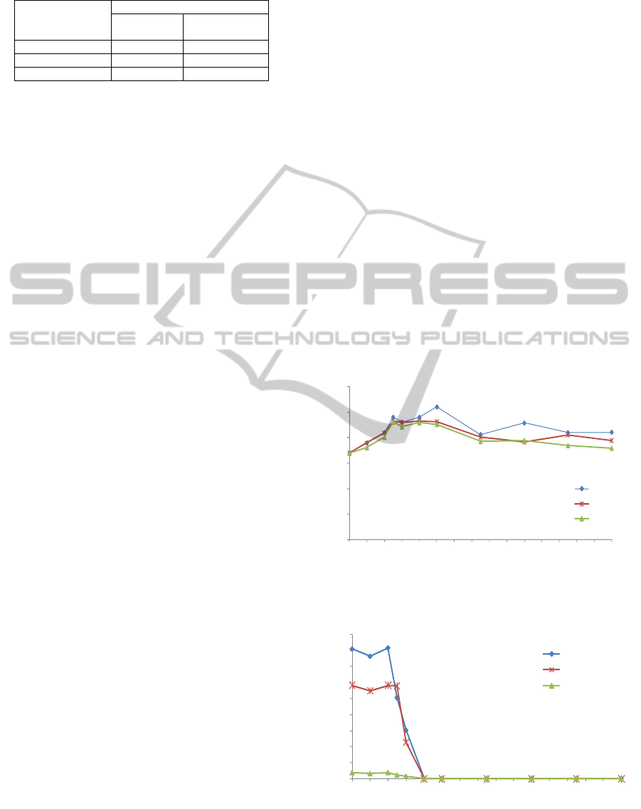
Table 2: Transformed risk degree of project.

project degree

of risk

Probabilit

error ran

Low

oun

High bound

low -5% +20%

medium -12.5% +35%

h -20% +50%

3 ANALYSIS OF THE

APPROPRIATE BN

CLOSENESS

The performance evaluation of the experimental

simulation results are summarized as follows:

 Throughput: representing the total throughput

of the all the completed projects during the

simulation period. As shown in Figure 2; when

the BN closeness rises at 75%, the project

throughput starts to rise considerably while it

significantly drops when the BN closeness is at

100%. In case of BN closeness at 100% and

low risks, the project throughputs (26) are

optimal, indicating that the throughputs are not

as high as expected (34) to fulfil our original

commitments. In general, in case of different

risk degrees, the BN closeness should be

controlled within 75%~100% to get the most

appropriate results.

 Delivery rate: representing the responsiveness

to meet the delivery time as designated by

customers. According to Figure 3 that the

delivery rate in case of different risks is better

when the BN closeness is lower than 75%,

indicating that the delivery responsiveness is

very poor when the BN closeness is higher than

75%.

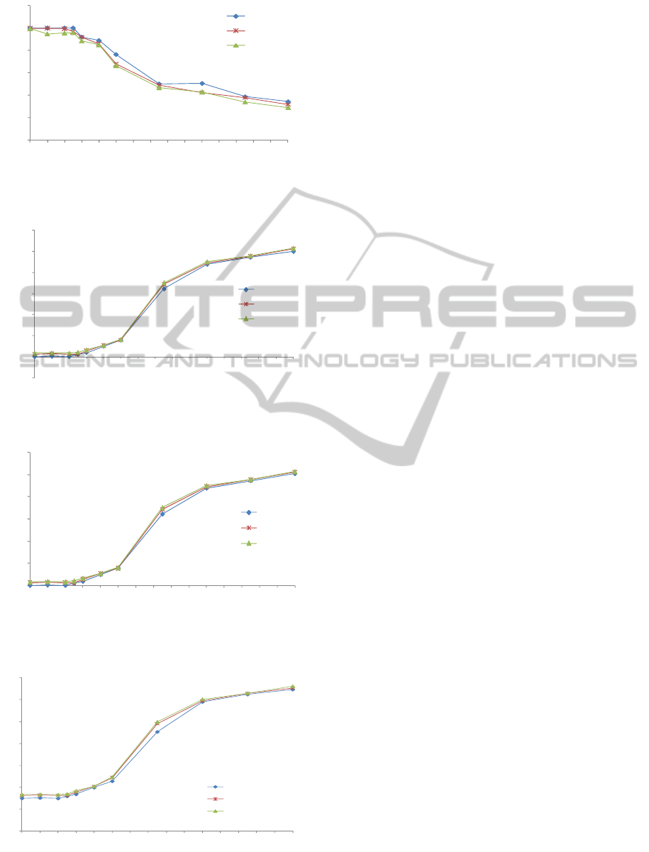
 Complete rate: representing the percentage of

completed projects in a multi-project

environment. As shown in Figure 4, in case of

different risks, the throughput rate will decrease

along with increasing BN closeness. When the

BN closeness accounting for more than 75%,

the complete rate declines, and the expected

number of completed projects will be

decreasing.

 Mean tardiness: tardiness refers to the delay

between the project completion time and

delivery time. The average value of the

tardiness of all projects is termed as the mean

tardiness. According to Figure 5, the mean

tardiness will rise along with increasing BN

closeness. In particular, the mean tardiness

starts to rise considerably when the BN

closeness accounting for more than 100%. This

indicates the project completion time cannot

satisfy demands on delivery accuracy and

become more serious when the BN closeness

accounting for more than 100%

 Mean lateness: lateness refers to the period that

the project completion time later than the due

delivery time. As seen in Figure 6 the mean

lateness time in case of different risks will rise

along with increasingly higher BN closeness.

And it becomes more and more serious when

the BN closeness accounting for more than

100% while it has no significant different when

the BN closeness accounting for less than 75%.

 Mean time in process: the equivalent of Time in

Process (TIP), namely, the time from project

opening to completion. As illustrated in Figure

7 mean TIP will rise along with rising BN

closeness. Higher BN closeness will result in

more serious bad multi-tasking and more

delivery delays of projects. However, it has no

significant difference when the BN closeness

accounting for less than 75%.

0.0

5.0

10.0

15.0

20.0

25.0

30.0

50%

60%

70%

80%

90%

100%

110%

120%

130%

140%

150%

160%

170%

180%

190%

200%

Throughputs

BN Closeness

Low risk

Medium risk

High risk

Figure 2: Project throughputs in case of different risk

degrees and BN closeness.

0.0

10.0

20.0

30.0

40.0

50.0

60.0

70.0

80.0

90.0

50%

60%

70%

80%

90%

100%

110%

120%

130%

140%

150%

160%

170%

180%

190%

200%

BN Closeness

Delivery Ra te (%)

Low risk

Medium risk

High risk

Figure 3: Delivery rate of BN closeness in case of

different risk degrees.

THE INFLUENCE ANALYSIS OF OPENING PROJECTS ON PROJECT PERFORMANCE

403

100

120

50%

60%

70%

80%

90%

100%

110%

120%

130%

140%

150%

160%

170%

180%

190%

200%

Complete Rate

(%)

BN Closeness

Low risk

Medium ris

High risk

Figure 4: Complete rate of BN closeness in case of

different risks.

-50.0

0.0

50.0

100.0

150.0

200.0

250.0

300.0

50%

60%

70%

80%

90%

100%

110%

120%

130%

140%

150%

160%

170%

180%

190%

200%

Mean Tardiness

(da ys)

BN Closeness

Low risk

Medium risk

High risk

Figure 5: Mean tardiness of BN closeness in case of

different risk degrees.

0.0

50.0

100.0

150.0

200.0

250.0

300.0

50%

60%

70%

80%

90%

100%

110%

120%

130%

140%

150%

160%

170%

180%

190%

200%

Mean Lateness

(da ys)

BN Closeness

Low risk

Medium risk

High risk

Figure 6: Mean lateness of BN closeness in case of

different risk degrees.

100

150

200

250

300

350

50%

60%

70%

80%

90%

100%

110%

120%

130%

140%

150%

160%

170%

180%

190%

200%

Mean TIP

(days)

BN Closeness

Low risk

Medium risk

High risk

Figure 7: Mean TIP of BN closeness in case of different

risk degrees.

4 CONCLUSIONS

The main purpose of this study is to get the most

appropriate degrees of BN closeness in uncertain

environment and verify the viewpoints of Dr.

Goldratt according to the experimental results. In

case of various risks, the setting of BN closeness at

75%~100% can result in better performance in terms

of the throughput, complete rate, delivery rate, mean

tardiness and mean lateness in the multi-project

environment. On the contrary, when increasing BN

closeness, the mean tardiness, mean lateness and

duration will increase.

ACKNOWLEDGEMENTS

The authors would like to thank the National

Science Council of the Republic of China for

financially supporting this research under Contract

NSC 99-2221-E-159-007.

REFERENCES

Adler, P. S., Mandelbaum, A., Nguyen, V. & Schwerer, E.,

1995, From project to process management: An

empirically-based framework for analyzing product

development time, Management Science, 41(3), 458.

Anavi-Isakow, S. & Golany, B., 2003, Managing multi-

project environments through constant work-in-

process, International Journal of Project Management,

21(1), 9-18.

Castro, J., Gómez, D. & Tejada, J., 2008, A rule for slack

allocation proportional to the duration in a PERT

network, European Journal of Operational Research,

187(2), 556-570.

Cates, G. R. & Mollaghasemi, M., 2007, The project

assessment by simulation technique, Engineering

Management Journal, December(1), 3-10.

Dietrich, P. & Lehtonen, P., 2005, Successful management

of strategic intentions through project - Reflections

from empirical study, International Journal of Project

Management, 23(5), 386-391.

Goldratt, E. M., 1997. Critical Chain . North-River Press.

Goldartt, E. M., 2006, The Strategy & Tactic Tree for

Projects.

Herroelen, W. & Leus, R., 2005, Project scheduling under

uncertainty: Survey and research potentials, European

Journal of Operational Research, 165(2), 289-306.

Shou, Y. & Yao, K. T., 2000, Estimation of project buffers

in critical chain project management, in Proceedings

of the 2000 IEEE International Conference on

Management of Innovation and Technology -- ICMIT

2000, 1(1), 162-167.

SIMULTECH 2011 - 1st International Conference on Simulation and Modeling Methodologies, Technologies and

Applications

404