
THE STABILITY BOX IN INTERVAL DATA FOR MINIMIZING
THE SUM OF WEIGHTED COMPLETION TIMES
Yuri N. Sotskov
United Institute of Informatics Problems, National Academy of Sciences of Belarus, Surganova Str 6, Minsk, Belarus
Natalja G. Egorova
United Institute of Informatics Problems, National Academy of Sciences of Belarus, Surganova Str 6, Minsk, Belarus
Tsung-Chyan Lai
Department of Business Administration, National Taiwan University, Roosevelt Rd 85, Taipei, Taiwan
Frank Werner
Faculty of Mathematics, Otto-von-Guericke-University, Magdeburg, Germany
Keywords:
Single-machine scheduling, Uncertain data, Total weighted flow time, Stability analysis.
Abstract:
We consider a single-machine scheduling problem, in which the processing time of a job can take any value
from a given segment. The criterion is to minimize the sum of weighted completion times of the n jobs, a
weight being associated with a job. For a job permutation, we study the stability box, which is a subset of
the stability region. We derive an O(nlogn) algorithm for constructing a job permutation with the largest
dimension and volume of a stability box. The efficiency of a permutation with the largest dimension and
volume of a stability box is demonstrated via a simulation on a set of randomly generated instances.
1 INTRODUCTION
In real-life scheduling, the numerical data are usu-
ally uncertain. A stochastic (Pinedo, 2002) or a fuzzy
method (Slowinski and Hapke, 1999) are used when
the job processing times may be defined as random
variables or as fuzzy numbers. If these times may
be defined neither as random variables with known
probability distributions nor as fuzzy numbers, other
methods are needed to solve a scheduling problem un-
der uncertainty (Daniels and Kouvelis, 1995; Sabun-
cuoglu and Goren, 2009; Sotskov et al., 2010b). The
robust method (Daniels and Kouvelis, 1995; Kasper-
ski, 2005; Kasperski and Zelinski, 2008) assumes that
the decision-makerprefers a schedule hedging against
the worst-case scenario. The stability method (Lai
and Sotskov, 1999; Lai et al., 1997; Sotskov et al.,
2009; Sotskov et al., 2010a; Sotskov et al., 2010b)
combines a stability analysis, a multi-stage decision
framework and a solution concept of a minimal dom-
inant set of semi-active schedules.
In this paper, we implement the stability method
for a single-machine problem with interval process-
ing times of the n jobs (Section 2). In Section 3, we
derive an O(nlogn) algorithm for constructing a job
permutation with the largest volume of a stability box.
Computational results are presented in Section 4. We
conclude with Section 5.
2 PROBLEM SETTING
Jobs J = {J
1
,..., J
n
}, n ≥ 2, have to be processed on
a single machine, a positive weight w
i
being given for
a job J
i
∈ J . The processing time p
i
of a job J
i
can
take any real value from a given segment [p
L
i
, p
U
i
], 0 ≤
p
L
i
≤ p
U
i
. The exact value p
i
∈ [p
L
i
, p
U
i
] may remain
unknown until the completion of job J
i
.
Let T = {p ∈ R
n
+
| p
L
i
≤ p
i
≤ p
U
i
, i ∈ {1, ...,n}}
denote the set of vectors p = (p
1
,... , p
n
) (scenarios)
of the possible job processing times. S = {π
1
,... ,π
n!
}
denotes the set of permutations π
k
= (J
k
1
,... ,J
k
n
) of
the jobs J . Problem 1|p
L
i
≤ p
i
≤ p
U
i
|
∑
w
i
C
i
is to find
an optimal permutation π
t
∈ S:
∑
J
i
∈J
w
i
C
i
(π
t
, p) = γ
t
p
= min
π
k
∈S
(
∑
J
i
∈J
w
i
C
i
(π
k
, p)
)
. (1)
14
N. Sotskov Y., G. Egorova N., Lai T. and Werner F..
THE STABILITY BOX IN INTERVAL DATA FOR MINIMIZING THE SUM OF WEIGHTED COMPLETION TIMES.
DOI: 10.5220/0003574400140023
In Proceedings of 1st International Conference on Simulation and Modeling Methodologies, Technologies and Applications (SIMULTECH-2011), pages
14-23
ISBN: 978-989-8425-78-2
Copyright
c
2011 SCITEPRESS (Science and Technology Publications, Lda.)

Hereafter,C
i
(π
k
, p) = C
i
is the completion time of job
J
i
∈ J in a semi-active schedule defined by permuta-
tion π
k
.
Since a factual scenario p ∈ T is unknown before
scheduling, the completion time C
i
of a job J
i
∈ J
can be determined only after the schedule execution.
Therefore, one cannot calculate the value γ
k
p
of the
objective function
γ =
∑
J
i
∈J
w
i
C
i
(π
k
, p)
for a permutation π
k
∈ S before the schedule realiza-
tion. However, one must somehow define a sched-
ule before to realize it. So, problem 1|p
L
i
≤ p
i
≤
p
U
i
|
∑
w
i
C
i
of finding an optimal permutation π
t
∈ S
defined in (1) is not correct. In general, one can find
only a heuristic solution (a job permutation) to prob-
lem 1|p
L
i
≤ p
i
≤ p
U
i
|
∑
w
i
C
i
the efficiency of which
may be estimated either analytically or via simulation.
In the deterministic case, when a scenario p ∈ T
is fixed before scheduling (i.e., equalities p
L
i
= p
U
i
=
p
i
hold for each job J
i
∈ J ), problem 1|p
L
i
≤ p
i
≤
p
U
i
|
∑
w
i
C
i
reduces to the classical problem 1||
∑
w
i
C
i
.
In contrast to the uncertain problem 1|p
L
i
≤ p
i
≤
p
U
i
|
∑
w
i
C
i
, problem 1||
∑
w
i
C
i
will be called deter-
ministic.
The deterministic problem 1||
∑
w
i
C
i
is correct and
can be solved exactly in O(nlogn) time (Smith, 1956)
due to the necessary and sufficient condition (2) for
the optimality of a permutation π
k
= (J
k
1
,... ,J
k
n
) ∈ S:
w
k
1
p
k
1
≥ . .. ≥
w
k
n
p
k
n
, (2)
where p
k
i
> 0 for each job J
k
i
∈ J . Using the suf-
ficiency of condition (2), problem 1||
∑
w
i
C
i
can be
solved to optimality by the weighted shortest process-
ing time rule: process the jobs J in non-increasing
order of their weight-to-process ratios
w
k
i
p
k
i
, J
k
i
∈ J .
3 THE STABILITY BOX
In (Sotskov and Lai, 2011), the stability box
S B (π
k
,T) within a set of scenarios T has been de-
fined for a permutation π
k
= (J
k
1
,... ,J
k
n
) ∈ S. To
present the definition of the stability box S B (π
k
,T),
we need the following notations.
We denote J (k
i
) = {J
k
1
,... ,J
k
i−1
} and J [k
i
] =
{J
k
i+1
,..., J
k
n
}. Let S
k
i
denote the set of permutations
(π(J (k
i
)),J
k
i
,π(J [k
i
])) ∈ S of the jobs J , π(J
′
) being
a permutation of the jobs J
′
⊂ J . Let N
k
denote a sub-
set of set N = {1, ...,n}. The notation 1|p|
∑
w
i
C
i
will
be used for indicating an instance with a fixed sce-
nario p ∈ T of the deterministic problem 1||
∑
w
i
C
i
.
Definition 1 (Sotskov and Lai, 2011). The maximal
closed rectangular box
S B (π
k
,T) = ×
k
i
∈N
k
[l
k
i
,u
k
i
] ⊆ T
is a stability box of permutation π
k
= (J
k
1
,... ,J
k
n
) ∈
S, if permutation π
e
= (J
e
1
,... ,J
e
n
) ∈ S
k
i
being op-
timal for the instance 1|p|
∑
w
i
C
i
with a scenario
p = (p
1
,... , p
n
) ∈ T remains optimal for the instance
1|p
′
|
∑
w
i
C
i
with a scenario
p
′
∈ {×
n
j=1, j6=i
[p
k
j
, p
k
j
]} × [l
k
i
,u
k
i
]
for each k
i
∈ N
k
. If there does not exist a scenario p ∈
T such that permutation π
k
is optimal for the instance
1|p|
∑
w
i
C
i
, then S B (π
k
,T) =
/
0.
The maximality of the closed rectangular box
S B (π
k
,T) = ×
k
i
∈N
k
[l
k
i
,u
k
i
]
in Definition 1 means that the box S B (π
k
,T) ⊆ T has
both a maximal possible dimension |N
k
| and a maxi-
mal possible volume.
For any scheduling instance, the stability box is
a subset of the stability region (Sotskov et al., 1998;
Sotskov et al., 2010a; Sotskov et al., 2010b). How-
ever, we substitute the stability region by the stability
box, since the latter is easy to compute (Sotskov et al.,
2010a; Sotskov and Lai, 2011).
In (Sotskov et al., 2010a), a branch-and-bound al-
gorithm has been developed to select a permutation
in the set S with the largest volume of a stability
box. If several permutations have the same volume of
the stability box, the algorithm from (Sotskov et al.,
2010a) selects one of them due to simple heuristics.
The efficiency of the constructed permutations has
been demonstrated on a set of randomly generated in-
stances with 5 ≤ n ≤ 100.
In (Sotskov and Lai, 2011), an O(nlogn) algo-
rithm has been developed for calculating a stability
box S B (π
k
,T) for the fixed permutation π
k
∈ S and
O(n
2
) algorithm has been developed for selecting a
permutation in the set S with the largest dimension
and volume of a stability box. The efficiency of these
algorithms was demonstrated on a set of randomly
generated instances with 10 ≤ n ≤ 1000.
All algorithms developed in (Sotskov et al.,
2010a; Sotskov and Lai, 2011) use the precedence-
dominance relation on the set of jobs J and the so-
lution concept of a minimal dominant set S(T) ⊆ S
defined as follows.
Definition 2 (Sotskov et al., 2009). The set of permu-
tations S(T) ⊆ S is a minimal dominant set for a prob-
lem 1|p
L
i
≤ p
i
≤ p
U
i
|
∑
w
i
C
i
, if for any fixed scenario
p ∈ T, the set S(T) contains at least one optimal per-
mutation for the instance 1|p|
∑
w
i
C
i
, provided that
any proper subset of set S(T) loses such a property.
THE STABILITY BOX IN INTERVAL DATA FOR MINIMIZING THE SUM OF WEIGHTED COMPLETION TIMES
15
Definition 3 (Sotskov et al., 2009). Job J
u
dominates
job J
v
, if there exists a minimal dominant set S(T) for
the problem 1|p
L
i
≤ p
i
≤ p
U
i
|
∑
w
i
C
i
such that job J
u
precedes job J
v
in every permutation of the set S(T).
Theorem 1 (Sotskov et al., 2009). For the problem
1|p
L
i
≤ p
i
≤ p
U
i
|
∑
w
i
C
i
, job J
u
dominates job J
v
if and
only if inequality (3) holds:
w
u
p
U
u
≥
w
v
p
L
v
. (3)
Due to Theorem 1 provenin (Sotskov et al., 2009),
we can obtain a compact presentation of a minimal
dominant set S(T) in the form of a digraph (J , A )
with the vertex set J and the arc set A . To this end,
we can check inequality (3) for each pair of jobs from
the set J and construct a dominance digraph (J ,A ) of
the precedence-dominance relation on the set of jobs
J as follows. The arc (J
u
,J
v
) belongs to the set A if
and only if inequality (3) holds. The construction of
the digraph (J ,A ) takes O(n
2
) time.
3.1 Illustrative Example
For the sake of simplicity of the calculation, we con-
sider a special case 1|p
L
i
≤ p
i
≤ p
U
i
|
∑
C
i
of problem
1|p
L
i
≤ p
i
≤ p
U
i
|
∑
w
i
C
i
when each job J
i
∈ J has a
weight w
i
equal to one. From condition (2), it follows
that a deterministic problem 1||
∑
C
i
can be solved to
optimality by the shortest processing time rule: pro-
cess the jobs in non-decreasing order of their process-
ing times p
k
i
, J
k
i
∈ J .
A set of scenarios T for Example 1 of the un-
certain problem 1|p
L
i
≤ p
i
≤ p
U
i
|
∑
C
i
is defined in
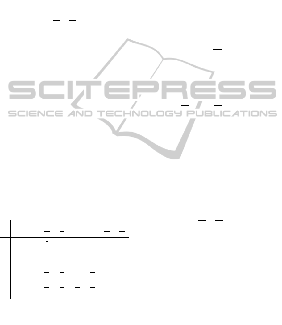
columns 1 and 2 in Table 1.
Table 1: Data for calculating S B (π
1
,T) for Example 1.
1 2 3 4 5 6 7 8
i p
L
i
p
U
i
w
i
p
U
i
w
i
p
L
i
d
−
i
d
+
i
w
i
d
+
i
w
i
d
−
i
1 2 3
1
3
0.5 1 0.5 2 1
2 1 9
1
9
1
1
6
1
3
3 6
3 8 8
1
8
1
8
1
6
1
9
9 6
4 6 10 0.1
1
6
0.1
1
9
9 10
5 11 12
1
12
1
11
0.1
1
11
11 10
6 10 19
1
19
0.1
1
15
1
12
12 15
7 17 19
1
19
1
17
1
15
1
19
19 15
8 15 20
1
20
1
15
1
20
1
19
19 20
In (Sotskov and Lai, 2011), formula (9) has been
proven. To use it for calculating the stability box
S B (π
k
,T), one has to define for each job J
k
i
∈ J the
maximal range [l
k
i
,u
k
i
] of possible variations of the
processing time p
k
i
preserving the optimality of per-
mutation π
k
(see Definition 1).
Due to the additivity of the objective function
γ =
∑
J
i
∈J
w
i
C
i
(π
k
, p),
the lower bound d
−
k
i
on the maximal range of possible
variations of the weight-to-process ratio
w
k
i
p
k
i
preserv-
ing the optimality of permutation π
k
= (J
k
1
,... ,J
k
n
) ∈
S is calculated as follows:
d
−
k
i
= max
(
w
k
i
p
U
k
i
, max
i< j≤n
(
w
k
j
p
L
k
j
))
,i ∈ {1,. . .,n−1}, (4)
d
−
k
n
=
w
k
n
p
U
k
n
. (5)
The upper bound d
+
k
i
,J
k
i
∈ J , on the maximal range of
possible variations of the weight-to-process ratio
w
k
i
p
k
i
preserving the optimality of permutation π
k
is calcu-
lated as follows:
d
+
k
i
= min
(
w
k
i
p
L
k
i
, min
1≤ j<i
(
w
k
j
p
U
k
j
))
,i ∈ {2, ...,n},
(6)
d
+
k
1
=
w
k
1
p
L
k
1
. (7)
For Example 1, the values d
−
k
i
,i ∈ {1, ...,8}, de-
fined in (4) and (5) are given in column 5 of Table
1. The values d
+
k
i
defined in (6) and (7) are given in
column 6.
In (Sotskov and Lai, 2011), the following claim
has been proven.
Theorem 2 (Sotskov and Lai, 2011). If there is no job
J
k
i
, i ∈ {1,. ..,n − 1}, in permutation π
k
= (J
k
1
,... ,
J
k
n
) ∈ S such that inequality
w
k
i
p
L
k
i
<
w
k
j
p
U
k
j
(8)
holds for at least one job J
k
j
, j ∈ {i+ 1, ...,n}, then
the stability box S B (π
k
,T) is calculated as follows:
S B (π
k
,T) = ×
d
−
k
i
≤d
+
k
i
"
w
k
i
d
+
k
i
,
w
k
i
d
−
k
i
#
. (9)
Otherwise, S B (π
k
,T) =
/
0.
Using Theorem 2, we can calculate the stability
box S B (π
1
,T) of permutation π
1
= (J
1
,... ,J
8
) in Ex-
ample 1. First, we convince that there is no job J
k
i
,
i ∈ {1,... ,n − 1}, with inequality (8). Due to Theo-
rem 2, S B (π
1
,T) 6=
/
0.
The bounds
w
k
i
d
+
k
i
and
w
k
i
d
−
k
i
on the maximal possible
variations of the processing times p
k
i
preserving the
optimality of permutation π
1
are given in columns 7
SIMULTECH 2011 - 1st International Conference on Simulation and Modeling Methodologies, Technologies and
Applications
16
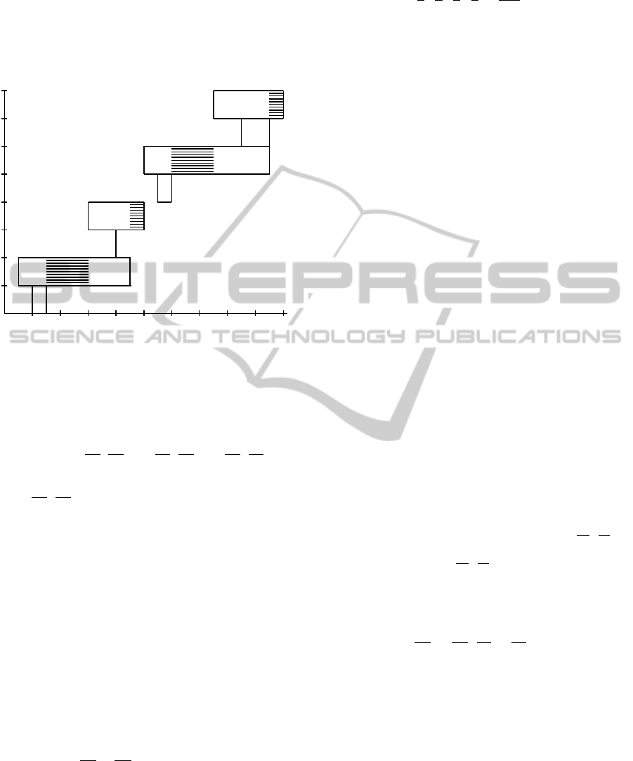
and 8 of Table 1. The maximal ranges (segments) of
possible variations of the job processing times within
the stability box S B (π
1
,T) are dashed in a coordinate
system in Fig. 1, where the abscissa axis is used for
indicating the job processing times and the ordinate
axis for the jobs from set J .
2 4 6 8 10 12 14 16 18 20
J
1
J
2
J
3
J
4
J
5
J
6
J
7
J
8
Figure 1: Maximal ranges [l
i
,u
i
] of possible variations of
the processing times p
i
,i ∈ {2,4, 6, 8}, within the stability
box S B (π
1
,T) are dashed.
Using formula (9), we obtain the stability box for
permutation π
1
as follows:
S B (π
1
,T) =
"
w
2
d
+
2
,
w
2
d
−
2
#
×
"
w
4
d
+
4
,
w
4
d
−
4
#
×
"
w
6
d
+
6
,
w
6
d
−
6
#
×
"
w
8
d
+
8
,
w
8
d
−
8
#
= [3, 6]× [9,10] ×[12,15] × [19,20].
Each job J
i
, i ∈ {1,3,5, 7}, has an empty range of pos-
sible variations of the time p
i
preserving the optimal-
ity of permutation π
1
since d
−
i
> d
+
i
(see columns 5
and 6 in Table 1). The dimension of the stability box
S B (π
1
,T) is equal to 4 = 8− 4. The volume of this
stability box is equal to 9 = 3· 1 · 3· 1.
In (Sotskov and Lai, 2011), O(nlogn) algorithm
STABOX has been developed for calculating the sta-
bility box S B (π
k
,T) for a fixed permutation π
k
∈ S.
For practice, the value of the relative volume of
a stability box is more useful than its absolute value.
The relative volume of a stability box is defined as the
product of the fractions
w
i
d
−
i
−
w
i
d
+
i
:
p
U
i
− p
L
i
(10)
for the jobs J
i
∈ J having non-empty ranges [l
i
,u
i
] of
possible variations of the processing time p
i
(inequal-
ity d
−
i
≤ d
+
i
must hold for such a job J
i
∈ J ).
The relative volume of the stability box for per-
mutation π
1
in Example 1 is calculated as follows:
3
8
·
1
4
·
3
9
·
1
5
=
1
160
.
The absolute volume of the whole box of the scenar-
ios T is equal to 2880 = 1· 8· 4·1·9·2· 5. The relative
volume of the rectangular box T is defined as 1.
3.2 Properties of a Stability Box
A job permutation in the set S with a larger dimension
and a larger volume of the stability box seems to be
more efficient than one with a smaller dimension and
(or) a smaller volume of stability box.
We investigate properties of a stability box, which
allow us to derive an O(nlogn) algorithm for choos-
ing a permutation π
t
∈ S which has
(a) the largest dimension |N
t
| of the stability box
S B (π
t
,T) = ×
t
i
∈N
t
[l
t
i
,u
t
i
] ⊆ T
among all permutations π
k
∈ S and
(b) the largest volume of the stability box
S B (π
t
,T) among all permutations π
k
∈ S having the
largest dimension |N
k
| = |N
t
| of their stability boxes
S B (π
k
,T).
Definition 1 implies the following claim.
Property 1. For any jobs J
i
∈ J and J
v
∈ J , v 6= i,
(w
i
/u
i
,w
i
/l
i
)
\
w
v
/p
U
v
,w
v
/p
L
v
= ∅.
Let S
max
denote the subset of all permutations π
t
in the set S possessing properties (a) and (b). Using
Property 1, we shall show how to define the relative
order of a job J
i
∈ J with respect to a job J
v
∈ J for
any v 6= i in a permutation π
t
= (J
t
1
,... ,J
t
n
) ∈ S
max
. To
this end, we have to treat all three possible cases (I)–
(III) for the intersection of the open interval
w
i
p
U
i
,
w
i
p
L
i
and the closed interval
h
w
v
p
U
v
,
w
v
p
L
v
i
. The order of the jobs
J
i
and J
v
in the desired permutation π
t
∈ S
max
may be
defined in the cases (I)–(III) using the following rules.
Case (I) is defined by the inequalities
w
v
p
U
v
≤
w
i
p
U
i
,
w
v
p
L
v
≤
w
i
p
L
i
(11)
provided that at least one of inequalities (11) is strict.
In case (I), the desired order of the jobs J
v
and J
i
in permutation π
t
∈ S
max
may be defined by a strict
inequality from (11): job J
v
proceeds job J
i
in permu-
tation π
t
. Indeed, if job J
i
proceeds job J
v
, then the
maximal ranges [l
i
,u
i
] and [l
v
,u
v
] of possible varia-
tions of the processing times p
i
and p
v
preserving the
optimality of π
k
∈ S are both empty (it follows from
equalities (4) – (7) and (9)).
Thus, the following property is proven.
Property 2. For case (I), there exists a permutation
π
t
∈ S
max
, in which job J
v
proceeds job J
i
.
THE STABILITY BOX IN INTERVAL DATA FOR MINIMIZING THE SUM OF WEIGHTED COMPLETION TIMES
17

Case (II) is defined by the equalities
w
v
p
U
v
=
w
i
p
U
i
,
w
v
p
L
v
=
w
i
p
L
i
. (12)
Property 3. For case (II), there exists a permutation
π
t
∈ S
max
, in which jobs J
i
and J
v
are located adja-
cently: i = t
r
and v = t
r+1
.
Proof. The maximal ranges [l
i
,u
i
] and [l
v
,u
v
] of pos-
sible variations of the processing times p
i
and p
v
pre-
serving the optimality of π
k
∈ S are both empty.
If job J
i
and job J
v
are located adjacently, then the
maximal range [l
u
,u
u
] of possible variation of the pro-
cessing time p
u
for any job J
u
∈ J \ {J
i
,J
v
} preserving
the optimality of permutation π
k
is no less than that if
at least one job J
w
∈ J \{J
i
,J
v
} is located between job
J
i
and job J
v
.
If equalities (12) hold, one can restrict the search
for a permutation π
t
∈ S
max
by a subset of permuta-
tions in set S with the adjacently located jobs J
i
and J
v
(Property 3). Moreover, the order of such jobs {J
i
,J
v
}
does not influence the volume of the stability box and
its dimension.
Remark 1. Due to Property 3, while looking for a
permutation π
t
∈ S
max
, we shall treat a pair of jobs
{J
i
,J
v
} satisfying (12) as one job (either job J
i
or J
v
).
Case (III) is defined by the strict inequalities
w
v
p
U
v
>
w
i
p
U
i
,
w
v
p
L
v
<
w
i
p
L
i
. (13)
For job J
i
∈ J satisfying case (III), let J (i) denote
the set of all jobs J
v
∈ J , for which the strict inequal-
ities (13) hold.
Property 4. (i) For a fixed permutation π
k
∈ S, job
J
i
∈ J may have at most one maximal segment [l
i
,u
i
]
of possible variations of the processing time p
i
∈
[p
L
i
, p
U
i
] preserving the optimality of permutation π
k
.
(ii) For the whole set of permutations S, only in
case (III), a job J
i
∈ J may have more than one
(namely: |J (i)| + 1 > 1) maximal segments [l
i
,u
i
] of
possible variations of the time p
i
∈ [p
L
i
, p
U
i
] preserv-
ing the optimality of this or that particular permuta-
tion from the set S.
Proof. Part (i) of Property 4 follows from the fact
that a non-empty maximal segment [l
i
,u
i
] (if any) is
uniquely determined by the subset J
−
(i) of jobs lo-
cated before job J
i
in permutation π
k
and the subset
J
+
(i) of jobs located after job J
i
. The subsets J
−
(i)
and J
+
(i) are uniquely determined for a fixed permu-
tation π
k
∈ S and a fixed job J
i
∈ J .
Part (ii) of Property 4 follows from the following
observations. If the open interval
w
i
p
U
i
,
w
i
p
L
i
does not intersect with the closed interval
w
v
p
U
v
,
w
v
p
L
v
for each job J
v
∈ J , then there exists a permuta-
tion π
t
∈ S
max
with a maximal segment [l
i
,u
i
] =
w
i
/p
U
i
,w
i
/p
L
i
preserving the optimality of permu-
tation π
t
.
Each job J
v
∈ J with a non-empty intersection
w
i
p
U
i
,
w
i
p
L
i
\
w
v
p
U
v
,
w
v
p
L
v
6=
/
0
satisfying inequalities (11) (case (I)) or equalities (12)
(case (II)) may shorten the above maximal segment
[l
i
,u
i
] and cannot generate a new possible maximal
segment.
In case (III), a job J
v
satisfying inequalities (13)
may generate a new possible maximal segment [l
i
,u
i
]
just for job J
i
satisfying the same strict inequalities
(13) as job J
v
does. So, the cardinality |L (i)| of the
whole set L (i) of such segments [l
i
,u
i
] is not greater
than |J (i)| + 1.
Let L denote the set of all maximal segments
[l
i
,u
i
] of possible variations of the processing times
p
i
for all jobs J
i
∈ J preserving the optimality of per-
mutation π
t
∈ S
max
. Using Property 4 and induction
on the cardinality |J (i)|, we proved
Property 5. |L | ≤ n.
3.3 A Job Permutation with the Largest
Volume of a Stability Box
The above properties allows us to derive an O(nlogn)
algorithm for calculating a permutation π
t
∈ S
max
with
the largest dimension |N
t
| and the largest volume of a
stability box S B (π
t
,T).
Algorithm MAX-STABOX
Input: Segments [p
L
i
, p
U
i
], weights w
i
, J
i
∈ J .
Output: Permutation π
t
∈ S
max
, stability box
S B (π
t
,T).
Step 1: Construct the list M (U) = (J
u
1
,... ,J
u
n
)
and the list W (U) = (
w
u
1
p
U
u
1
,... ,
w
u
n
p
U
u
n
)
in non-decreasing order of
w
u
r
p
U
u
r
.
Ties are broken via increasing
w
u
r
p
L
u
r
.
Step 2: Construct the list M (L) = (J
l
1
,... ,J
l
n
)
and the list W (L) = (
w
l
1
p
L
l
1
,...,
w
l
n
p
L
l
n
)
in non-decreasing order of
w
l
r
p
L
l
r
.
Ties are broken via increasing
w
l
r
p
U
l
r
.
Step 3: FOR j = 1 to j = n DO
SIMULTECH 2011 - 1st International Conference on Simulation and Modeling Methodologies, Technologies and
Applications
18

compare job J
u
j
and job J
l
j
.
Step 4: IF J
u
j
= J
l
j
THEN job J
u
j
has to be
located in position j in permutation
π
t
∈ S
max
GOTO step 8.
Step 5: ELSE job J
u
j
= J
i
satisfies inequalities
(13). Construct the set J (i) = {J
u
r+1
,... ,
J
l
k+1
} of all jobs J
v
satisfying
inequalities (13), where J
i
= J
u
j
= J
l
k
.
Step 6: Choose the largest range [l
u
j
,u
u
j
]
among those generated for job J
u
j
= J
i
.
Step 7: Partition the set J (i) into subsets J
−
(i)
and J
+
(i) generating the largest range
[l
u
j
,u
u
j
]. Set j = k + 1 GOTO step 4.
Step 8: Set j := j + 1 GOTO step 4.
END FOR
Step 9: Construct the permutation π
t
∈ S
max
via
putting the jobs J in the positions defined
in steps 3 – 8.
Step 10: Construct the stability box S B (π
t
,T)
using algorithm STABOX derived in
(Sotskov and Lai, 2011). STOP.
Steps 1 and 2 of algorithm MAX-STABOX are
based on Property 3 and Remark 1. Step 4 is based
on Property 2. Steps 5 – 7 are based on Property 4,
part (ii). Step 9 is based on Property 6 which follows.
To proveProperty 6, we have to analyze algorithm
MAX-STABOX. In steps 1, 2 and 4, all jobs J
t
=
{J
i
| J
u
j
= J
i
= J
l
j
} having the same position in both
lists M (U) and M (L) obtain fixed positions in the
permutation π
t
∈ S
max
.
The positions of the remaining jobs J \ J
t
in the
permutation π
t
are determined in steps 5 – 7. The
fixed order of the jobs J
t
may shorten the original seg-
ment [p
L
i
, p
U
i
] of a job J
i
∈ J \ J
t
as follows: [ bp
L
i
, bp
U
i
].
So, in steps 5 – 7, the reduced segment [bp
L
i
, bp
U
i
] has
to be considered instead of segment [p
L
i
, p
U
i
] for a job
J
i
∈ J \ J
t
. Let I
′
denote the maximal subset of set I
including exactly one element from each set I(i), for
which job J
i
∈ J satisfies the strict inequalities (13).
Property 6. There exists a permutation π
t
∈ S with
the set I
′
⊆ I of maximal segments [l
i
,u
i
] of possible
variations of the processing time p
i
,J
i
∈ J , preserving
the optimality of permutation π
t
.
Proof. Due to Property 2 and steps 1 – 4 of algo-
rithm MAX-STABOX, the maximal segments [l
i
,u
i
]
and [l
v
,u
v
] (if any) of jobs J
i
and J
v
satisfying (11)
preserve the optimality of permutation π
t
∈ S
max
.
Let J
∗
denote the set of all jobs J
i
satisfying (13).
It is easy to see that
\
J
i
∈J
(bp
L
i
, bp
U
i
] = ∅.
Therefore,
\
J
i
∈J
J (i) = ∅.
Hence, step 9 is correct: putting the set of jobs J in
the positions defined in steps 3 – 8 does not cause any
contradiction of the job orders.
Obviously, steps 1 and 2 take O(nlogn) time. Due
to Properties 4 and 5, steps 6, 7 and 9 take O(n)
time. Step 10 takes O(nlogn) time since algorithm
STABOX derived in (Sotskov and Lai, 2011) has the
same complexity. Thus, the whole algorithm MAX-
STABOX takes O(nlogn) time.
It is easy to convince that, due to steps 1 –
5, permutation π
t
constructed by algorithm MAX-
STABOX possesses property (a) and, due to steps 6,
7 and 9, this permutation possesses property (b).
Remark 2. Algorithm MAX-STABOX constructs a
permutation π
t
∈ S such that the dimension |N
t
| of
the stability box S B (π
t
,T) = ×
t
i
∈N
t
[l
t
i
,u
t
i
] ⊆ T is the
largest one for all permutations S, and the volume
of the stability box S B (π
t
,T) is the largest one for
all permutations π
k
∈ S having the largest dimension
|N
k
| = |N
t
| of their stability boxes S B (π
k
,T).
Returning to Example 1, one can show (using
Algorithm MAX-STABOX) that permutation π
1
=
(J
1
,... ,J
8
) has the largest dimension and volume of
a stability box. Next, we compare S B (π
1
,T) with
the stability boxes calculated for the permutations ob-
tained by the three heuristics defined as follows.
The lower-point heuristic generates an optimal
permutation π
l
∈ S for the instance 1|p
L
|
∑
w
i
C
i
with
p
L
= (p
L
1
,... , p
L
n
) ∈ T. (14)
The upper-point heuristic generates an optimal
permutation π
u
∈ S for the instance 1|p
U
|
∑
w
i
C
i
with
p
U
= (p
U
1
,..., p
U
n
) ∈ T. (15)
The mid-point heuristic generates an optimal per-
mutation π
m
∈ S for the instance 1|p
M
|
∑
w
i
C
i
with
p
M
=
p
U
1
− p
L
1
2
,... ,
p
U
n
− p
L
n
2
∈ T. (16)
We obtain the permutation π
l
= (J
2
,J
1
,J
4
,J
3
,J
6
,
J
5
,J
8
,J
7
) with the stability box
S B (π
l
,T)=
w
2
d
+
2
,
w
2
d
−
2
×
w
6
d
+
6
,
w
6
d
−
6
=[1, 2]×[10,11].
The volume of the stability box S B (π
l
,T) is
equal to 1. We obtain the permutation π
u
= (J
1
,J
3
,
J
2
,J
4
,J
5
,J
7
,J
6
,J
8
) and the permutation π
m
= (J
1
,J
2
,
J
4
,J
3
,J
5
,J
6
,J
8
,J
7
). The volume of the stability box
S B (π
u
,T)=
w
4
d
+
4
,
w
4
d
−
4
×
w
8
d
+
8
,
w
8
d
−
8
=[9,10]×[19,20]
THE STABILITY BOX IN INTERVAL DATA FOR MINIMIZING THE SUM OF WEIGHTED COMPLETION TIMES
19

is equal to 1. The volume of the stability box
S B (π
m
,T)=
w
2
d
+
2
,
w
2
d
−
2
×
w
6
d
+
6
,
w
6
d
−
6
=[3, 6]×[12,15]
is equal to 9 = 3·3. It is the same volume of the stabil-
ity box as that of permutation π
1
. Note, however, that
the dimension |N
m
| of the stability box S B (π
m
,T) is
equal to 2, while the dimension |N
1
| of the stability
box S B (π
1
,T) of the permutation π
1
∈ S
max
is equal
to 4. Thus, π
m
6∈ S
max
since permutation π
m
does not
possess property (a).
4 COMPUTATIONAL RESULTS
There might be several permutations with the largest
dimension and relative volume of a stability box
S B (π
t
,T) since several consecutive jobs in a permu-
tation π
t
∈ S
max
may have an empty range of possi-
ble variations of their processing times preserving the
optimality of permutation π
t
. In the computational
experiments, we break ties in ordering such jobs by
adopting the mid-point heuristic which generates a
subsequence of these jobs as a part of an optimal per-
mutation π
m
∈ S for the instance 1|p
M
|
∑
w
i
C
i
with the
scenario p
M
∈ T defined by (16).
Our choice of the mid-point heuristic is based
on the computational results of the experiments con-
ducted in (Sotskov and Lai, 2011) for the problem
1|p
L
i
≤ p
i
≤ p
U
i
|
∑
w
i
C
i
with 10 ≤ n ≤ 1000. In those
computational results, the subsequence of a permu-
tation π
m
∈ S outperformed both the corresponding
subsequence of permutation π
l
∈ S and that of permu-
tation π
u
∈ S defined by (14) and (15), respectively.
We coded the algorithm MAX-STABOX com-
bined with the mid-point heuristic for ordering con-
secutive jobs having an empty range of their process-
ing times preserving the optimality of permutation
π
t
∈ S
max
in C++. This algorithm was tested on a
PC with AMD Athlon (tm) 64 Processor 3200+, 2.00
GHz, 1.96 GB of RAM. We solved (exactly or ap-
proximately) a lot of randomly generated instances.
Some of the computational results obtained are pre-
sented in Tables 2 and 3 for randomly generated in-
stances of the problem 1|p
L
i
≤ p
i
≤ p
U
i
|
∑
w
i
C
i
with
the number n ∈ { 1000, 1100,...,2000} of jobs.
Each series presented in Tables 2 and 3 contains
100 solved instances with the same combination of
the number n of jobs and the same maximal possi-
ble error δ% of the random processing times p
i
∈
[p
L
i
, p
U
i
]. An integer center C of a segment [p
L
i
, p
U
i
]
was generated using the uniform distribution in the
range [L,U]: L ≤ C ≤ U. The lower bound p
L
i
for the
possible job processing time p
i
∈ [p
L
i
, p
U
i
] was defined
as
p
L
i
= C· (1−
δ
100
),
the upper bound p
U
i
of p
i
∈ [p
L
i
, p
U
i
] was defined as
p
U
i
= C · (1+
δ
100
).
The same range [L,U] for the varying center
C of the segment [p
L
i
, p
U
i
] was used for all jobs
J
i
∈ J , namely: L = 1 and U = 100. In Ta-
bles 2 and 3, we report computational results for
series of instances of the problem 1|p
L
i
≤ p
i
≤
p
U
i
|
∑
w
i
C
i
with the maximal possible errors δ%
of the job processing times from the set {0.25%,
0.4%,0.5%,0.75%,1%,2.5%,5%, 15%,25%}.
For each job J
i
∈ J , the weight w
i
∈ R
1
+
was uni-
formly distributed in the range [1,50]. It should be
noted that the job weights w
i
were assumed to be
known before scheduling (in contrast to the actual
processing times p
∗
i
of the jobs J
i
∈ J , which were
assumed to be unknown before scheduling).
The number n of jobs in each instance of a series
is given in column 1 of Table 2 and Table 3. The
maximum possible error δ% of the random processing
times p
i
∈ [p
L
i
, p
U
i
] is given in column 2.
Column 3 represents the average relative number
|A | of the arcs in the dominance digraph (J ,A ) con-
structed using condition (3) of Theorem 1. The rel-
ative number |A | is calculated in percentages of the
number of arcs in the complete circuit-free digraph of
order n as follows:
|A | :
n(n− 1)
2
· 100%.
Column 4 represents the averagedimension |N
t
| of
the stability box S B (π
t
,T) of the permutation π
t
with
the largest relative volume of a stability box. |N
k
| is
equal to the number of jobs with a non-zero maximal
possible variation of the processing time preserving
the optimality of permutation π
t
∈ S
max
. Column 5
represents the average relative volume of the stability
box S B (π
t
,T) of the permutations π
t
with the largest
dimension and relative volume of a stability box. If
S B (π
t
,T) = T for all instances in the series, then col-
umn 5 contains number one.
In the experiments, we answered the question of
how large the relative error ∆ of the objective func-
tion γ =
∑
n
i=1
w
i
C
i
was for the permutation π
t
∈ S
max
with the largest dimension and relative volume of a
stability box S B (π
t
,T):
∆ =
γ
t
p
∗
− γ
p
∗
γ
p
∗
,
where p
∗
is the actual scenario (unknown before
scheduling), γ
p
∗
is the optimal objective function
value for scenario p
∗
∈ T and γ
t
p
∗
=
∑
n
i=1
w
i
C
i
(π
t
, p
∗
).
SIMULTECH 2011 - 1st International Conference on Simulation and Modeling Methodologies, Technologies and
Applications
20

Table 2: Randomly generated instances with [L,U] = [1,100], w
i
∈ [1,50] and n ∈ {1000,1100,.. . ,1500}.
Number Maximal Relative Average Relative Number Average Maximal CPU
of jobs error of p
i
arc number dimension volume of of exact error error time
n δ% |A | (in %) |N
t
| S B (π
t
,T) solutions ∆ ∆ (in s)
1 2 3 4 5 6 7 8 9
1000 0.25% 100 1000 1 100 0 0 8.62
1000 0.4% 100 1000 1 100 0 0 8.56
1000 0.5% 100 989.61 0.227427 11 ≈ 0 ≈ 0 8.69
1000 0.75% 99.545177 451.29 ≈ 0 0 0.000023 0.000031 8.98
1000 1% 99.192559 330.65 ≈ 0 0 0.000042 0.000051 8.96
1000 2.5% 97.591726 124 0.000001 0 0.000157 0.000181 8.9
1000 5% 94.889794 54.86 0.001976 0 0.000526 0.000614 8.84
1000 15% 84.39185 12.29 0.011288 0 0.004309 0.004858 8.86
1000 25% 73.954372 4.71 0.09081 0 0.012045 0.013303 8.89
1100 0.25% 100 1100 1 100 0 0 11.51
1100 0.4% 100 1100 1 100 0 0 11.46
1100 0.5% 99.997839 1087.27 0.200252 11 ≈ 0 ≈ 0 11.51
1100 0.75% 99.539967 478.35 ≈ 0 0 0.000023 0.00003 12.1
1100 1% 99.188722 349.3 ≈ 0 0 0.000043 0.000049 12.05
1100 2.5% 97.611324 131.01 0.000001 0 0.000155 0.000175 11.8
1100 5% 94.862642 57.35 0.006242 0 0.000528 0.000593 11.79
1100 15% 84.288381 11.46 0.017924 0 0.004371 0.004899 11.76
1100 25% 74.076585 4.29 0.133804 0 0.01189 0.013289 11.8
1200 0.25% 100 1200 1 100 0 0 15.4
1200 0.4% 100 1200 1 100 0 0 15.12
1200 0.5% 99.998 1185.27 0.174959 5 ≈ 0 0.000001 15.42
1200 0.75% 99.540619 515.8 ≈ 0 0 0.000023 0.000029 16
1200 1% 99.190977 375.34 ≈ 0 0 0.000042 0.000051 16.06
1200 2.5% 97.581479 138.75 0.000002 0 0.000156 0.000177 15.81
1200 5% 94.88253 62.06 0.006396 0 0.000534 0.000596 15.51
1200 15% 84.376763 12.88 0.042597 0 0.004332 0.004733 15.33
1200 25% 74.100395 5.01 0.08078 0 0.011872 0.01351 15.21
1300 0.25% 100 1300 1 100 0 0 19.75
1300 0.4% 100 1300 1 100 0 0 19.38
1300 0.5% 99.997583 1280.26 0.084004 2 ≈ 0 ≈ 0 19.54
1300 0.75% 99.549162 543.2 ≈ 0 0 0.000023 0.000026 20.3
1300 1% 99.199789 400.41 ≈ 0 0 0.000042 0.000053 20.32
1300 2.5% 97.602491 148.41 0.000004 0 0.000157 0.000186 20.01
1300 5% 94.877326 65.23 0.019927 0 0.000532 0.000588 19.95
1300 15% 84.388473 13.47 0.024207 0 0.004364 0.004758 19.52
1300 25% 73.975873 5.5 0.08254 0 0.011962 0.013812 19.52
1400 0.25% 100 1400 1 100 0 0 24.92
1400 0.4% 100 1400 1 100 0 0 24.8
1400 0.5% 99.997556 1377.21 0.078809 1 ≈ 0 0.000001 24.97
1400 0.75% 99.539142 575.2 ≈ 0 0 0.000023 0.000029 25.67
1400 1% 99.198461 422.65 ≈ 0 0 0.000042 0.00005 25.63
1400 2.5% 97.594897 154.9 0.000001 0 0.000157 0.000178 25.1
1400 5% 94.869044 70.36 0.002356 0 0.000533 0.000615 25.29
1400 15% 84.364242 14.35 0.029338 0 0.004339 0.004841 24.72
1400 25% 74.096446 5.18 0.14077 0 0.011998 0.013041 24.27
1500 0.25% 100 1500 1 100 0 0 31.44
1500 0.4% 100 1500 1 100 0 0 31.08
1500 0.5% 99.997493 1474.09 0.070241 0 ≈ 0 0.000001 31.64
1500 0.75% 99.544441 607.5 ≈ 0 0 0.000042 0.000052 32.39
THE STABILITY BOX IN INTERVAL DATA FOR MINIMIZING THE SUM OF WEIGHTED COMPLETION TIMES
21

Table 3: Randomly generated instances with [L,U] = [1,100], w
i
∈ [1,50] and n ∈ {1500,1600,.. . ,2000}.
Number Maximal Relative Average Relative Number Average Maximal CPU
of jobs error of p
i
arc number dimension volume of of exact error error time
n δ% |A | (in %) |N
t
| S B (π
t
,T) solutions ∆ ∆ (in s)
1500 1% 99.193199 444.29 ≈ 0 0 0.000042 0.000052 32.39
1500 2.5% 97.61593 167.25 0.000005 0 0.000155 0.000171 31.43
1500 5% 94.861654 71.34 0.00282 0 0.000533 0.000582 31.36
1500 15% 84.409904 14.93 0.05372 0 0.004394 0.00492 30.46
1500 25% 74.281235 5.46 0.148403 0 0.011936 0.013685 30.33
1600 0.25% 100 1600 1 100 0 0 38.63
1600 0.4% 100 1600 1 100 0 0 38.67
1600 0.5% 99.997452 1569.35 0.046151 0 ≈ 0 0.000001 38.8
1600 0.75% 99.54273 638.18 ≈ 0 0 0.000023 0.00003 39.76
1600 1% 99.192323 464.89 ≈ 0 0 0.000042 0.000048 40.04
1600 2.5% 97.601128 174.91 0.000004 0 0.000157 0.000177 38.71
1600 5% 94.861356 76.990000 0.003505 0 0.000532 0.000581 38.46
1600 15% 84.343239 14.75 0.036278 0 0.004341 0.004811 37.34
1600 25% 74.123830 5.75 0.087651 0 0.011899 0.013192 36.34
1700 0.25% 100 1700 1 100 0 0 47.29
1700 0.4% 100 1700 1 100 0 0 47.18
1700 0.5% 99.997432 1665.41 0.034556 1 ≈ 0 0.000001 47.12
1700 0.75% 99.544993 671.09 ≈ 0 0 0.000023 0.000027 48.25
1700 1% 99.203930 495.13 ≈ 0 0 0.000041 0.000049 48.47
1700 2.5% 97.598734 180.99 0.000072 0 0.000156 0.000172 46.88
1700 5% 94.852439 80.53 0.001601 0 0.000533 0.000585 46.33
1700 15% 84.358524 17.27 0.028854 0 0.004379 0.0049 45.26
1700 25% 74.030579 6.03 0.082325 0 0.012069 0.013255 44.24
1800 0.25% 100 1800 1 100 0 0 56.18
1800 0.4% 100 1800 1 100 0 0 56.27
1800 0.5% 99.99761 1764.02 0.02624 0 ≈ 0 0.000001 56.72
1800 0.75% 99.547537 706.21 ≈ 0 0 0.000023 0.000028 57.38
1800 1% 99.193797 517.06 ≈ 0 0 0.000042 0.000049 57.33
1800 2.5% 97.600247 190.97 0.000042 0 0.000156 0.000177 55.81
1800 5% 94.899074 84.82 0.007274 0 0.000529 0.000602 55.27
1800 15% 84.408342 17.67 0.040758 0 0.004348 0.004723 53.42
1800 25% 74.162869 6.38 0.126377 0 0.011981 0.013095 51.86
1900 0.25% 100 1900 1 100 0 0 65.65
1900 0.4% 100 1900 1 100 0 0 66.81
1900 0.5% 99.997533 1858.51 0.018832 0 ≈ 0 0.000001 66.69
1900 0.75% 99.54191 733.81 ≈ 0 0 0.000023 0.000028 67.75
1900 1% 99.189512 534.79 ≈ 0 0 0.000042 0.000049 68.58
1900 2.5% 97.596318 199.82 0.000022 0 0.000156 0.000173 66.36
1900 5% 94.856400 89.93 0.002011 0 0.000534 0.000596 65.68
1900 15% 84.331351 17.61 0.048813 0 0.004372 0.004844 62.97
1900 25% 74.188836 6.82 0.092068 0 0.011965 0.013234 60.74
2000 0.25% 100 2000 1 100 0 0 78.41
2000 0.4% 100 2000 1 100 0 0 78.93
2000 0.5% 99.997489 1953.88 0.017798 2 ≈ 0 ≈ 0 79.06
2000 0.75% 99.542435 764.35 ≈ 0 0 0.000023 0.000027 78.83
2000 1% 99.197383 565.09 ≈ 0 0 0.000042 0.000048 78.1
2000 2.5% 97.605895 210.17 0.000035 0 0.000156 0.000173 75.8
2000 5% 94.867102 93.63 0.014015 0 0.000535 0.000606 75.02
2000 15% 84.412199 17.95 0.040101 0 0.004339 0.004751 74.08
2000 25% 73.977021 6.64 0.147426 0 0.01203 0.013046 71.22
SIMULTECH 2011 - 1st International Conference on Simulation and Modeling Methodologies, Technologies and
Applications
22

Column 6 represents the number of instances
(among the 100 instances in a series) for which a per-
mutation π
t
with the largest dimension and relative
volume of the stability box S B (π
t
,T) provides an op-
timal solution for the instance 1|p
∗
|
∑
w
i
C
i
with the
actual processing times p
∗
= (p
∗
1
,... , p
∗
n
) ∈ T. From
the experiments, it follows that, if the maximal pos-
sible error of the processing times is no greater than
0.4%, then the dominance digraph (J ,A ) is a com-
plete circuit-free digraph. Therefore, the permutation
π
t
∈ S
max
provides an optimal solution for the instance
1|p
∗
|
∑
w
i
C
i
.
The average (maximum) relative error ∆ of the ob-
jective function value γ
t
p
∗
calculated for the permu-
tation π
t
∈ S
max
constructed by the algorithm MAX-
STABOX with respect to the optimal objective func-
tion value γ
p
∗
defined for the actual job processing
times is givenin column 7 (in column 8, respectively).
For all series presented in Tables 2 and 3, the aver-
age (maximum) error ∆ of the value γ
t
p
∗
of the objec-
tive function γ =
∑
n
i=1
w
i
C
i
obtained for the permu-
tation π
t
∈ S
max
with the largest dimension and rel-
ative volume of a stability box was not greater than
0.012069 (not greater than 0.013812).
The CPU-time for an instance of a series is pre-
sented in column 5. This time includes the time for
the realization of the O(n
2
) algorithm for construct-
ing the dominance digraph (J ,A ) using condition (3)
of Theorem 1 and the time for the realization of the
O(nlogn) algorithm MAX-STABOX for construct-
ing the permutation π
t
∈ S
max
and the stability box
S B (π
t
,T). This CPU-time grows rather slowly with
n, and it was not greater than 79.06 s for each instance.
5 CONCLUSIONS
In (Sotskov and Lai, 2011), an O(n
2
) algorithm has
been developed for calculating a permutation π
t
∈ S
with the largest dimension and volume of a stabil-
ity box S B (π
t
,T). In Section 3, we proved Proper-
ties 1 – 6 of a stability box allowing us to derive an
O(nlogn) algorithm for calculating such a permuta-
tion π
t
∈ S
max
. The dimension and volume of a sta-
bility box are efficient invariants of uncertain data T,
as it is shown in simulation experiments on a PC re-
ported in Section 4.
ACKNOWLEDGEMENTS
The first and third authors were supported in this re-
search by National Science Council of Taiwan.
REFERENCES
Daniels, R. and Kouvelis, P. (1995). Robust scheduling
to hedge against processing time uncertainty in single
stage production. Management Science, V. 41(2):363–
376.
Kasperski, A. (2005). Minimizing maximal regret in
the single machine sequencing problem with maxi-
mum lateness criterion. Operations Research Letters,
V. 33:431–436.
Kasperski, A. and Zelinski, P. (2008). A 2-approximation
algorithm for interval data minmax regret sequencing
problem with total flow time criterion. Operations Re-
search Letters, V. 36:343–344.
Lai, T.-C. and Sotskov, Y. (1999). Sequencing with uncer-
tain numerical data for makespan minimization. Jour-
nal of the Operations Research Society, V. 50:230–
243.
Lai, T.-C., Sotskov, Y., Sotskova, N., and Werner, F. (1997).
Optimal makespan scheduling with given bounds of
processing times. Mathematical and Computer Mod-
elling, V. 26(3):67–86.
Pinedo, M. (2002). Scheduling: Theory, Algorithms, and
Systems. Prentice-Hall, Englewood Cliffs, NJ, USA.
Sabuncuoglu, I. and Goren, S. (2009). Hedging production
schedules against uncertainty in manufacturing envi-
ronment with a review of robustness and stability re-
search. International Journal of Computer Integrated
Manufacturing, V. 22(2):138–157.
Slowinski, R. and Hapke, M. (1999). Scheduling un-
der Fuzziness. Physica-Verlag, Heidelberg, Germany,
New York, USA.
Smith, W. (1956). Various optimizers for single-stage
production. Naval Research Logistics Quarterly,
V. 3(1):59–66.
Sotskov, Y., Egorova, N., and Lai, T.-C. (2009). Minimizing
total weighted flow time of a set of jobs with interval
processing times. Mathematical and Computer Mod-
elling, V. 50:556–573.
Sotskov, Y., Egorova, N., and Werner, F. (2010a). Mini-
mizing total weighted completion time with uncertain
data: A stability approach. Automation and Remote
Control, V. 71(10):2038–2057.
Sotskov, Y. and Lai, T.-C. (2011). Minimizing total
weighted flow time under uncertainty using domi-
nance and a stability box. Computers & Operations
Research. doi:10.1016/j.cor.2011.02.001.
Sotskov, Y., Sotskova, N., Lai, T.-C., and Werner, F.
(2010b). Scheduling under Uncertainty. Theory and
Algorithms. Belorusskaya nauka, Minsk, Belarus.
Sotskov, Y., Wagelmans, A., and Werner, F. (1998). On
the calculation of the stability radius of an optimal or
an approximate schedule. Annals of Operations Re-
search, V. 83:213–252.
THE STABILITY BOX IN INTERVAL DATA FOR MINIMIZING THE SUM OF WEIGHTED COMPLETION TIMES
23
