STOCHASTIC MODELLING IN HEALTHCARE SYSTEMS
Srinivas R. Chakravarthy
Department of Industrial and Manufacturing Engineering, Kettering University, MI-48504, Flint, U.S.A.
Keywords: Healthcare system, Applied stochastic modelling, Markovian arrival process, Phase type distribution,
simulation, and ARENA.
Abstract: We are at a point in time where healthcare (in USA) is getting more attention from law makers, government
agencies, doctors, hospitals, pharmaceutical companies, and population at large. The costs for healthcare
have been steadily growing. The healthcare system offers challenging and interesting opportunities for
operations researchers from both theoretical and practical points of view. This paper is an attempt to use
simulation as a tool to study a healthcare system at a macroscopic level.
1 INTRODUCTION
With baby-boomers growing at a faster rate and the
required workforce (to support the existing older
people and the boomers) dwindling in size, the
United States healthcare system (HCS) is receiving
attention at every level. The country is facing multi-
dimensional problems with regards to HCS. On one
hand the worry is to make sure that everyone living
in this country has an affordable health insurance.
For way too long this has been largely ignored in
spite of the constant exposure of this problem.
Obviously, one of the main reasons is the cost
associated with making everyone insured. Hence,
insured people as well as the governmental (both
local and federal) agencies have been putting up the
bill on the uninsured. While some are uninsured due
to their own choice, majority of them cannot afford
to pay for their insurance. With the current economic
condition the problem is even more exacerbated. On
the other hand, HCS has so much waste (Thomson
Reuters, 2009, Washington Post, 2009) that a small
percentage of the savings will pay for the costs
associated with the uninsured patients. In fact, if
done properly the overall costs can be significantly
brought down. For example, identifying the areas of
wastage, underutilized resources, and needing
significant improvement, will help this cause.
According to a white paper published by
Thomson Reuters, 2009, the U.S. HCS wastes
between $600 billion and $850 billion annually. This
is about one-third of the nation’s healthcare bill.
This report identifies a number of categories (in
broader terms) where wastage occurs (see Figure 1
below). About 40% of the wastage is estimated
under the “unnecessary care” category.
This is defined as “Unwarranted treatment, such
as the over-use of antibiotics and the use of
diagnostic lab tests to protect against malpractice
exposure, accounts for $250 billion to $325 billion
in annual healthcare spending.”
Figure 1: Percentage of waste in US HCS.
One of the items mentioned in the 40% category
is the “use of diagnostic lab tests”. Diagnostic labs
cover a wide range of labs such as blood test, X-
rays, MRI, and Cardio. In an ideal world a patient
requiring any type of lab test should be able to get it
without having to wait for excessively long period of
time. But as we all know this is not the case for a
variety of reasons. These (not necessarily in any
order) are: (a) lack of resources; (b) improper
allocation of resources; (c) scheduling of patients;
and (d) queuing delays due to unexpected arrivals.
109
R. Chakravarthy S..
STOCHASTIC MODELLING IN HEALTHCARE SYSTEMS.
DOI: 10.5220/0003576101090115
In Proceedings of 1st International Conference on Simulation and Modeling Methodologies, Technologies and Applications (SIMULTECH-2011), pages
109-115
ISBN: 978-989-8425-78-2
Copyright
c
 2011 SCITEPRESS (Science and Technology Publications, Lda.)

We are in an era where the competition is so strong.
As technology grows exponentially, both the
patients and the doctors would like to use the
technology to cure the patients efficiently and in a
short period of time. Hence, a HCS would like to
attract and enrol more patients and the doctors to its
organization. One of the ways of doing this is to
provide “quality” service at an affordable price and
still make profit. Note that a typical HCS consists of
many (major) groups such as (a) administrative; (b)
doctors who serve the patients insured through the
system; (c) hospitals that serve the patients covered
by the system and (d) laboratories that serve the
hospitals, doctors, and patients. It should be noted
that there may be interactions between these groups.
For example, some hospitals have their own
laboratories which serve the patients admitted to the
hospital either as in-patients or out-patients. Most
doctors visit hospitals to take care of not only their
own patients but also other patients who have been
admitted. We will not model that aspect in this
paper.
The study of such systems in which most of the
underlying variables are random falls in the area of
stochastic modelling and one can avail the tools
therein to study healthcare models. However,
tracking analytically the system performance
measures such as the mean waiting times and the
utilization factors is almost infeasible due to inherent
complexities and the significant interactions that are
present among various segments of a healthcare
system. An alternative approach to analytical
modelling is through simulation. While simulation in
healthcare has evolved at a slow pace (as compared
to other non-healthcare systems such as
manufacturing and telecommunications) over the
last three decades or so (see e.g., Jun, et al., 1999,
Baldwin, et al., 2004), it is recognized as an
important tool in solving problems arising in
healthcare systems. Most of the published papers
dealing with simulation in healthcare systems focus
on sub-systems such as emergency room, outpatient
clinics, etc. (Eldabi, et al., 2010, Gunal and Pidd,
2010). For latest developments in simulation and its
application to many fields including healthcare
systems we refer the reader to journals such as
Simulation Modelling Practice and Theory,
Simulation in Healthcare, Journal of Simulation, and
Proceedings of Winter Simulation Conference.
Thus, the objective of this paper is to provide
insights into how stochastic modelling can be
applied to a typical HCS at a macroscopic level so as
to help the management with aggregate planning. It
is our intent here to focus on the use of simulation to
identify bottlenecks that cause excessive delays in
patients receiving service, and areas of under
utilization of the resources, by looking at a HCS at a
macroscopic level. More specific ones (within this
type of HCS) requiring microscopic level modelling
will be addressed elsewhere.
2 MODEL DESCRIPTION
As indicated earlier a HCS is plagued with wastage,
underutilized resources, and excessive delays
experienced by patients. Whether one is dealing with
handling patients to go through diagnostic labs or to
process paperwork before (and after) the patients go
through diagnostics or the doctors to notify the
patients of the results, or the patients need to be
admitted in the hospitals, or the patients requiring
operations need to wait for beds, equipments,
personnel, delays are inevitable due to available
finite resources and the way they are allocated
among competing service providers. These delays
are further compounded by inherent randomness.
For example, the arrivals of the patients to service
providers are not deterministic. Different classes of
patients arrive and they have to be attended based on
their priorities. These are also random. The service
times are usually random and some patients may
have to go through the same service more than once
for reasons that cannot be anticipated. Thus, a
natural approach to solving such problems is the use
of stochastic modelling. While analytical modelling
is important, there are instances such as the current
study where one has to rely on simulation due to
complex nature of the model.
Patients are the central focus in any HCS and so
we start with assuming that patients arrive to a HCS
according to a Markovian arrival process (MAP)
with representation (D
0
, D
1
) of order m. Note that
the transitions corresponding to no arrivals are
governed by D
0
and the transitions corresponding to
arrivals are governed by D
1
. The underlying
continuous-time Markov chain (CTMC) has the
generator given by Q = D
0
+D
1
. This representation
of MAP is a special case of batch Markovian arrival
process (BMAP). This BMAP was originally
introduced by Neuts (1979) as a versatile Markovian
point process in 1979. MAP, a very versatile point
process used extensively in stochastic modelling,
includes several well-known point processes such as
Poisson, Erlang, and hyperexponential. For full
details on MAP and its applications to stochastic
models we refer to (Lucantoni, 1991, Chakravarthy,
2001, Chakravarthy, 2010). The fundamental rate
(the rate of arrivals per unit of time), λ, is given by
SIMULTECH 2011 - 1st International Conference on Simulation and Modeling Methodologies, Technologies and
Applications
110

,eπ
1
D=
λ
where π is the steady state probability
vector of the generator Q governing the underlying
CTMC satisfying πQ = 0, πe = 1 and where e is a
column vector of 1’s with dimension m.
While one can model the arrivals of different
priority type patients to follow independent MAPs,
we choose here to model the arrivals to be dependent
on each other generated by a common MAP with an
associated probability vector. However, it is easy to
modify our model to accommodate any variation to
the current one. Also, the idea of using MAP to
model patient arrivals is to incorporate inherent
correlation present in the inter-arrival times of
patients.
Note that the patients in any HCS require
different types of services. Thus, the patients are
classified based on their service requirements that
range from a simple administrative query to a more
serious one requiring key resources such as doctors,
labs, etc. We assume that a HCS under consideration
has N groups and that with probability p
i
, 1 ≤ i ≤ N,
an arriving patient belongs to group i and let p = (p
1
,
p
2
,…, p
N
). We will, henceforth, refer to them as
patients of type i. Type i patients have to go through
K
i
stages of servicing. This is again typical of a
HCS. For example, a patient admitted into a hospital
has to go through registration, triage, examination
room, etc. Also, patients who call administrative
people for any query related to billing, office visits,
and other activities go through various stages before
hanging up the phone.
We assume that the service times of patients of
type i, 1 ≤ i ≤ N, need to go through K
i
stages and in
each stage the time required to process the patients is
of phase type. (A phase type distribution (PH-
distribution) is obtained as the time until absorption
in a finite state continuous time Markov chain with n
transient states and one absorbing states. Thus, a PH
distribution is represented by (
β , S) of order n. PH-
distributions include well-known distributions such
as exponential, (generalized) Erlang, and
hyperexponentials as very special cases (Neuts,
1995).
These stages represent the patients going through
admission process, filling necessary paperwork,
triage, etc. It is possible for some patients to seek
direct or indirect services from another group after
getting serviced in the group they entered. For
example, patients getting into hospitals may have to
seek administrative help for follow up paperwork or
examination/billing details. Some may opt to ask at a
later point in time (in which case we can treat them
as new arrivals to the system) or as part of their
current visit. We model this scenario by specifying
the routing mechanism. We also put a restriction that
a patient may not seek services from more than two
groups (including the one that was entered). This is
not only to mimic the most practical situations but
also to avoid patients cycling through many groups
more than once. This one requires more book-
keeping. A pictorial description of this model is
displayed in Figure 2.
Thus, the processing time of a priority i patient
in stage j, 1 ≤ j ≤ K
i
, 1 ≤ i ≤ N, is assumed to be of
phase type with representation (β(i,j), S(i, j)) of order
n
ij
.
MAP arrivals
GROUP1
GROUP2
GROUPN
Figure 2: A typical HCS.
By keeping track of the phase of the arrival
process, the number of type i patients in the system,
and the phase of the services in various stages, one
can study the model under consideration using
Markov chain theory and algorithmic methods
(Neuts, 1989, 1995). However, the state space for
the model grows exponentially and the book-
keeping is very involved. Furthermore, the
computations of the distributions of the waiting
times in the system of patients are very complicated
to describe analytically. Thus, we will use
simulation to study our model. We have chosen
ARENA to simulate the model under study.
2.1 Simulation with ARENA
In this section we will outline how ARENA is used
to simulate the HCS under study. The following
assumptions are made in developing the model in
ARENA.
(a) The number of groups and the number of stages
within each group are as follows:
N = 4, K
1
= 2, K
2
= 2, K
3
= 3, and K
4
= 5.
(b) Type 1 patients go through both their stages and
then leave the system after getting the services.
STOCHASTIC MODELLING IN HEALTHCARE SYSTEMS
111

(c) Type 2 patients go through both stages before
leaving the system.
(d) Type 3 patients go through one of the three
sequences: (i) Stage 1 to Stage 2 to Stage 3; (ii)
Stage 1 to Stage 2; (iii) Stage 1 to Stage 3; according
to a probability vector, say, p
2
= (p
21
, p
22
, p
23
)
before leaving the system.
(e) Type 4 patients go through one of the five
sequences: (i) Stage 1 to Stage 2 to Stage 3 to Stage
4 to Stage 5; (ii) Stage 1 to Stage 2 to Stage 5; (iii)
Stage 1 to Stage 5; (iv) Stage 1 to Stage 2 to Stage 4
to Stage 5; and (v) Stage 1 to Stage 2 to Stage 3 to
Stage 5; according to a probability vector, say, p
3
=
(p
31
, p
32
, p
33
, p
34
, p
35
) before leaving the system.
(f) Patients of types 2, 3, and 4 create additional
work for servers in Stage 2 of Group 1 when they
leave the system. These have a lower priority as
compared to Type 1 patients.
3 ILLUSTRATIVE EXAMPLE
For our illustrative example, we consider five
different arrival processes and different service time
distributions. The five arrival processes with
parameter matrices D
0
and D
1
are as follows. The
base time units are taken to be minutes.
EXPA: Exponential: D
0
= -1and D
1
= 1.
ERLA: Erlang of order 5

01
5 5 0 0 0 00000
0 5 5 0 0 00000
,.
0 0 5 5 0 00000
0 0 0 5 5 00000
0 0 0 0 5 50000
DD
−
⎡⎤⎡⎤
⎢⎥⎢⎥
−
⎢⎥⎢⎥
⎢⎥⎢⎥
==
−
⎢⎥⎢⎥
−
⎢⎥⎢⎥
⎢⎥⎢⎥
−
⎣⎦⎣⎦
HEXA: Hyperexponential: This is the mixture of
two exponential with mixing probabilities 0.9 and
0.1, and with parameters 1.9 and 0.19. Here
.
019.0171.0
190.0710.1
,
19.00
09.1
10
⎥
⎦
⎤
⎢
⎣
⎡
−
=
⎥
⎦
⎤
⎢
⎣
⎡
−
−
= DD
MNCA: MAP with negatively correlated arrivals:
Here we take D
0
and D
1
to be

01
1.00222 1.00222 0 0 0 0
0 1.00222 0 , 0.01002 0 0.9922 .
0 0 225.75 223.4925 0 2.2575
DD
−
⎡⎤⎡⎤
⎢⎥⎢⎥
=− =
⎢⎥⎢⎥
⎢⎥⎢⎥
−
⎣⎦⎣⎦
MPCA: MAP with positively correlated arrivals:
Here we take D
0
and D
1
to be

01
1.00222 1.00222 0 0 0 0
0 1.00222 0 , 0.9922 0 0.01002 .
0 0 225.75 2.2575 0 223.4925
DD
−
⎡⎤⎡⎤
⎢⎥⎢⎥
=− =
⎢⎥⎢⎥
⎢⎥⎢⎥
−
⎣⎦⎣⎦
All these five MAP processes are normalized
during simulation so as to have an arrival rate of
12/minute. However, these are qualitatively different
in that they have different variance and correlation
structure. The first three arrival processes, namely
ERLA, EXPA, and HEXA, correspond to renewal
processes and so the correlation is 0. The arrival
process labeled MNCA has correlated arrivals with
correlation between two successive inter-arrival
times given by -0.4889 and the arrivals
corresponding to the processes labeled MPCA has a
positive correlation with values 0.4889. The ratio of
the standard deviations of the inter-arrival times of
these five arrival processes with respect to ERLA
are, respectively, 1, 2.2361, 5.0194, 3.1518, and
3.1518.
For services in various stages in different groups
we pick among the following three special cases of
PH-distributions. These are displayed in general
notations and in the examples we will point out the
specific values used for these parameters.
EXPS: Exponential:
β = (1) , S = (- ξ).
ERLS(µ, m): Erlang of order m
.)0,...,0,1(
⎥
⎥
⎥
⎥
⎦
⎤
⎢
⎢
⎢
⎢
⎣
⎡
−
−
−
==
μ
μμ
μμ
β
%
S
HEXS(β,µ): This is the mixture of two exponential
with mixing probabilities β = (β
1
,…, β
m
) and with
parameters µ = (µ
1
,…, µ
m
). These parameters will be
chosen so as to arrive at a desired mean.
.),...,(
2
1
1
⎥
⎥
⎥
⎥
⎦
⎤
⎢
⎢
⎢
⎢
⎣
⎡
−
−
−
==
m
m
S
μ
μ
μ
βββ
%
All three PH-distributions will be normalized by
modifying the parameters so as to have a specific
mean. However, these are qualitatively different in
that they have different variance structure. Note that
the coefficient of variation of ERLS, EXPS, and
HEXS are, respectively, less than 1, equal to 1 and
greater than 1.
In Table 1 we list the values of the parameters of
the model under study used in simulation. In the
following we denote Stage j in Group i by G
i
S
j
, for
1 ≤ j ≤ K
i
, 1 ≤ i ≤ N.
Before we specify other parameters of the model,
we display in Figure 3 the bar diagram of some key
statistics (related to our model) taken from various
SIMULTECH 2011 - 1st International Conference on Simulation and Modeling Methodologies, Technologies and
Applications
112

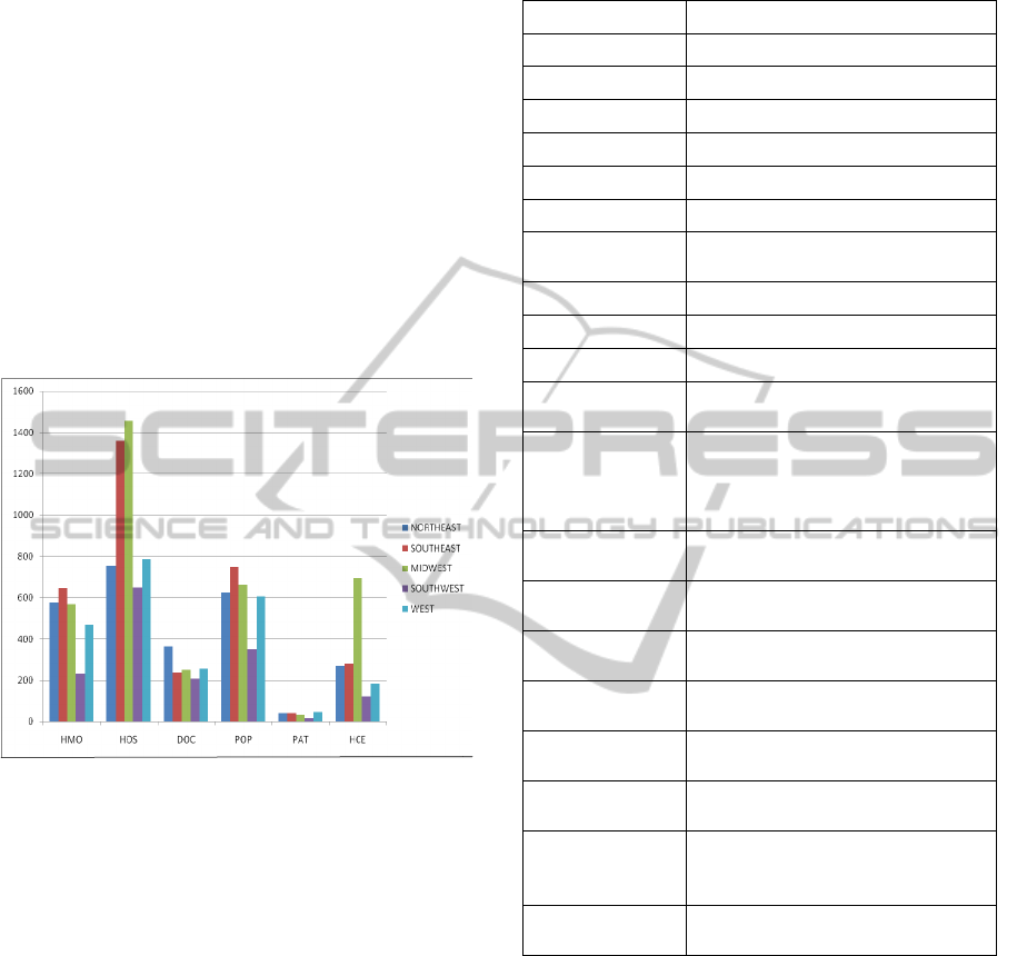
sources such as state health facts (SHF), US Census
(Census), and population by state that are available
on the public domain. We first group the 50 states
and the District of Columbia of USA into 5 regions
as: (a) Northeast consisting of 13 states; (b)
Southeast with 12 states; (c) Midwest with 12 states;
(d) Southwest with 4 states; and (e) West with 10
states. The number of HMOs (HMO) and the
number of hospitals (HOS) are in actual units; the
units for doctors (DOC) are the rate per 100,000
residents; the population (POP) is in units of
100,000s; the number of patients (PAT) served by
Federally-funded Federally qualified health centers
are in units of 100,000s, and the number of
healthcare employees (HCE) are in 100,000s.
Figure 3: Key statistics related to a HCS.
It should be noted that such statistics pertaining
to specific HMOs or hospitals or doctors or any
other category may not only be proprietary in nature
but also difficult to obtain. So, we try our best to
reasonably estimate the parameters for our
simulation model. Also this is the first step that we
take in dealing with modelling a healthcare system
at the macroscopic level (mainly for aggregate
planning) and hence there is room for considerable
improvement in the future.
In the following let c
ij
, 1 ≤ j ≤ K
i
, 1 ≤ i ≤ N,
denote the number of service providers such as
doctors or healthcare administrative personnel, etc.,
available to serve type i patients in Stage j. Based on
the statistics seen above coupled with additional
statistics on one of the local HMOs we fix our other
parameters as follows. All the time units are in
minutes. The simulation was run for 365 days on a
24-hr basis. In Tables 2 through 4 we display the (a)
utilization of resources; (b) mean and (c) coefficient
of variation (CV) of the waiting time in the system.
Table 1: Parameter values.
Parameter Values
N 4
(K
1
, K
2
, K
3
, K
4
) (2, 2, 3, 5 )
λ
5/minute
(c
11
, c
12
) (20, 40)
(c
21
, c
22
) (500, 250)
(c
31
, c
32
, c
33
) (40, 30, 30)
(c
41
, c
42
, c
43
, c
44
,
c
45
)
(50, 75, 125, 150, 200)
p (0.1, 0.6, 0.2, 0.1)
p
2
(0.30, 0.35, 0.35)
p
3
(0.1, 0.2, 0.2, 0.2, 0.3)
Service time at
G
1
S
1
ERLS(0.2, 5)
Service time at
G
1
S
2
HEXS ((0.6,0.3,0.1),(0.68, 0.068,
0.0068)) for type 1 patients;
ERLS(1/0.3,10) for additional
work
Service time at
G
2
S
1
ERLS(1/3, 5)
Service time at
G
2
S
2
HEXS ((0.85,0.1,0.05),(0.3425,
0.03425, 0.003425)
Service time at
G
3
S
1
ERLS(1/3, 5)
Service time at
G
3
S
2
ERLS(2.5, 5)
Service time at
G
3
S
3
ERLS(1, 5)
Service time at
G
4
S
1
ERLS(0.25, 5)
Service time at
G
4
S
2
, G
4
S
3
,
G
4
S
4
, and G
4
S
5
HEXS ((0.85,0.1,0.05),(0.17125
0.017125, 0.0017125)
MAP ERLA, EXPA, HEXA, MNCA,
MPCA
Looking at these tables we notice that all arrival
processes have pretty much the same utilization in
all sectors. The utilization is not high for any of the
sectors. In fact, the largest value is 0.590. With
regards to the mean waiting time in the system, we
find that the five arrival processes appear to have
similar values for all types of patients. However,
with respect to the additional paperwork (created by
types 2, 3, and 4 patients) the mean time taken is
much higher for the positively correlated arrivals. In
fact, the mean is almost three times as large as the
other arrival processes.
The CV of the waiting time in the system of
patients shows a different pattern as compared to the
mean waiting time for the five arrival processes
STOCHASTIC MODELLING IN HEALTHCARE SYSTEMS
113

considered. For example, the smallest value for CV
seems to occur for type 3 patients with positively
correlated arrivals. This measure, for type 3 patients,
is larger than 1 in all cases indicating that standard
deviation of the waiting time in the system to be
much larger than the mean.
Table 2: Utilization of the resources.
MAP ERLA EXPA HEXA MNCA MPCA
G
1
S
1
0.251 0.250 0.249 0.250 0.251
G
1
S
2
0.590 0.583 0.584 0.587 0.588
G
2
S
1
0.090 0.090 0.090 0.090 0.090
G
2
S
2
0.240 0.240 0.239 0.240 0.238
G
3
S
1
0.374 0.375 0.375 0.375 0.374
G
3
S
2
0.067 0.067 0.067 0.067 0.067
G
3
S
3
0.166 0.166 0.166 0.167 0.166
G
4
S
1
0.200 0.200 0.200 0.200 0.200
G
4
S
2
0.271 0.269 0.264 0.263 0.270
G
4
S
3
0.161 0.160 0.157 0.158 0.159
G
4
S
4
0.135 0.131 0.134 0.133 0.133
G
4
S
5
0.100 0.099 0.099 0.100 0.101
Table 3: Mean waiting time in the system.
MAP ERLA EXPA HEXA MNCA MPCA
Type 1 30.23 29.64 29.83 29.91 31.43
Type 2 34.99 35.01 34.94 34.98 34.83
Type 31 22.02 22.01 22.00 22.03 24.77
Type 32 22.00 22.03 22.01 22.00 24.78
Type 33 21.98 22.01 22.02 21.99 24.81
Type 41 185.84 175.79 180.16 181.02 180.31
Type 42 181.60 180.57 179.38 180.24 179.83
Type 43 177.86 179.46 178.96 178.08 183.42
Type 44 180.56 179.82 177.87 177.34 180.10
Type 45 181.50 179.43 178.97 177.81 179.42
Paperwork 3.00 3.00 3.00 3.00 8.80
Table 4: CV of the waiting time in the system.
MAP ERLA EXPA HEXA MNCA MPCA
Type 1 0.471 0.470 0.472 0.470 0.490
Type 2 0.385 0.382 0.383 0.383 0.385
Type 31 3.086 3.095 3.078 3.078 2.463
Type 32 3.084 3.090 3.087 3.094 2.479
Type 33 3.086 3.075 3.083 3.088 2.470
Type 41 0.498 0.501 0.488 0.499 0.491
Type 42 0.490 0.486 0.494 0.495 0.493
Type 43 0.497 0.497 0.498 0.491 0.498
Type 44 0.496 0.490 0.505 0.494 0.495
Type 45 0.494 0.500 0.495 0.492 0.498
Paperwork 0.316 0.316 0.316 0.316 1.631
In the case of additional paperwork, we notice
that CV is about 5 times larger for the positively
correlated arrivals as compared to all the other
arrivals (which all have roughly the same value).
This illustrates that one cannot solely depend on the
means. In practice, the management normally uses
the means to allocate appropriate resources and this
example points out the danger in doing so.
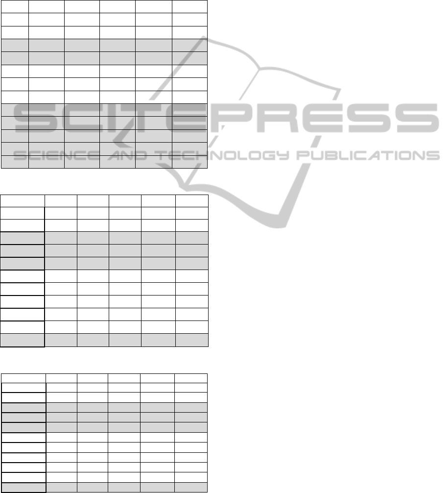
Finally, we display the fitted distributions of the
waiting times of different patients in various stages
in Table 5. In most applications the waiting time
distribution will be skewed to the right since some
patients have to wait unusually longer than the
others. Therefore, we notice that most of the fitted
distributions are either gamma, lognormal, or beta,
which are very common in situations that exhibit a
large variation. In the case of all but positively
correlated arrival processes, we observe that the best
fit for the time spent by the additional paperwork is
same as the processing time (Erlang of order 10 with
parameter 10/3). This indicates that the additional
paperwork is processed soon after its arrival.
However, for the positively correlated this is not the
case and there appears to exhibit a large variation
requiring a beta distribution. Thus, in practice one
should integrate fully the type of distribution used
for the arrivals rather than just a few descriptive
measures such as mean, standard deviation, and
correlation.
4 CONCLUSIONS
In this paper we used ARENA simulation software
to study a healthcare system at a macroscopic level
and identified a few underutilized resources as well
as areas for improvement (with regards to delay in
waiting for services). We used a versatile point
process to model the arrivals of patients and phase
type distributions for the services of the patients in
various stages of a HCS. Different types of patients
require different sequencing to get services and are
routed accordingly. It should be pointed out that the
intent of this paper is not to simulate any specific
unit of a HCS but to highlight the need (especially
for aggregate planning) for modelling at a
macroscopic level through an example. Thus, in this
first attempt the results are only approximate and
should be taken and interpreted carefully. There are
several variants and improvements to the current
model and will be addressed elsewhere.
SIMULTECH 2011 - 1st International Conference on Simulation and Modeling Methodologies, Technologies and
Applications
114

Table 5: Fitted distributions of the waiting time in the system (using ARENA notation).
ERLA EXPA HEXA MNCA MPCA
Type 1 2 + LOGN(22.4, 29.4) 2 + LOGN(22, 28.5) 1 + LOGN(22.9, 26.9) 1 + LOGN(22.9, 26.9) 1 + LOGN(24.7, 28.7)
Type 2 3 + LOGN(23.9, 25.5) 2 + LOGN(24.8, 24.4) 2 + LOGN(24.8, 24.4) 2 + LOGN(24.8, 24.4) 2 + LOGN(24.7, 24.3)
Type 31 5 + GAMM(3.06, 5.57) 5 + GAMM(3.05, 5.58) 5 + GAMM(3.07, 5.54) 5 + GAMM(3.07, 5.55) 5 + GAMM(4.59, 4.31)
Type 32 5 + GAMM(3.07, 5.55) 5 + GAMM(3.06, 5.56) 4 + GAMM(2.83, 6.36) 4 + GAMM(2.82, 6.39) 5 + GAMM(4.54, 4.35)
Type 33 5 + GAMM(3.06, 5.56) 5 + GAMM(3.08, 5.53) 5 + GAMM(3.06, 5.56) 5 + GAMM(3.05, 5.57) 5 + LOGN(19.9, 10.6)
Type 41 8 + LOGN(140, 244) 8 + LOGN(132, 221) 8 + LOGN(133, 227) 8 + LOGN(136, 233) 7 + LOGN(135, 225)
Type 42 8 + LOGN(135, 232) 8 + LOGN(133, 229) 7 + LOGN(134, 223) 7 + LOGN(135, 226) 8 + LOGN(134, 228)
Type 43 7 + LOGN(134, 222) 8 + LOGN(135, 228) 7 + LOGN(135, 224) 7 + LOGN(133, 220) 8 + LOGN(137, 238)
Type 44 7 + LOGN(135, 226) 8 + LOGN(133, 226) 8 + LOGN(134, 227 8 + LOGN(133, 224) 7 + LOGN(135, 224)
Type 45 7 + LOGN(136, 228) 6 + LOGN(136, 221) 6 + LOGN(135, 219) 6 + LOGN(134, 217) 8 + LOGN(134, 228)
Paperwork ERLA(0.3, 10) ERLA(0.3, 10) ERLA(0.3, 10) ERLA(0.3, 10) 152 * BETA(0.296, 4.82)
REFERENCES
Baldwin, L.P., Eldabi, T., Paul, R. J., 2004. Simulation in
healthcare management: a soft approach (MAPIU).
Simulation Modeling Practice and Theory, 12,
541-557.
Chakravarthy, S. R. 2001., The Batch Markovian Arrival
Process: A Review and Future Work. In Advances in
Probability Theory and Stochastic Processes, Eds., A.
Krishnamoorthy, N. Raju, and V. Ramaswami, 21-49.
Notable Publications, Inc., New Jersey, USA.
Chakravarthy, S. R., 2010. Markovian Arrival Process.
Wiley Encyclopedia of Operations Research and
Management Science. Published Online: 15 JUN
2010.
Eldabi, T., Jun, G.T., Clarkson, J., Connell, C., and Klein,
J. H. 2010. Model driven healthcare: disconnected
practices. Proceedings of the 2010 Winter Simulation
Conference. B. Johansson, S. Jain, J. Montoya-Torres,
J. Hugan, and E. Yücesan, eds., 2271-2282
Gunal, M. M., Pidd, M., 2010. Discrete event simulation
for performance modelling in health care: a review of
the literature. Journal of Simulation, 42-51.
Jun, J. B., Jacobson, S. H., Swisher, J. R., 1999.
Application of discrete-event simulation in health care
and clinics: a survey, Journal of the Operational
Research Society, 50, 109–123.
Lucantoni, D. 1991. New results on the single server
queue with a batch Markovian arrival process.
Stochastic Models, 7, 1-46.
Neuts, M. F. 1995. Matrix-Geometric Solutions in
Stochastic Models -An Algorithmic Approach. Dover
Publications, Mineola, NY, USA. (originally
published by Johns Hopkins University Press, 1981).
Neuts, M. F. 1979. A versatile Markovian point process. J.
Appl. Prob., 16, 764-779.
Neuts, M. F. 1989. Structured Stochastic Matrices of
M/G/1 type and their 1applications. Marcel Dekker,
New York, NY, USA.
Census http://www.census.gov/statab/ranks/rank18.html
(March 25, 2011)
Infoplease http://www.infoplease.com/ipa/A0004986.html
(March 25, 2011)
Thomson Reuters, 2009. http://thomsonreuters.com/
content/press_room/tsh/waste_US_healthcare_system
(March 18, 2011).
Washington Post, 2009. http://media.washingtonpost.com/
wp-/nation/pdf/healthreport_092909.pdf (March 18,
2001).
SHF. www.statehealthfacts.org (March 25, 2011)
STOCHASTIC MODELLING IN HEALTHCARE SYSTEMS
115