MULTI-SCALE APPROACH TO POPULATION BALANCE

MODELLING OF DISPERSE SYSTEMS

Béla G. Lakatos

Institute of Process Engineering, University of Pannonia, Egyetem Street 10, Veszprém, Hungary

Keywords: Disperse systems, Multi-scale modelling, Population balance, Crystallization, Two-population model.

Abstract: A three-scale model is presented and analysed using the multi-scale methodology of complex systems. The

micro-scale model is formulated as a set of stochastic differential equations for the individual disperse

objects and it is shown that the population balance equation, containing also terms describing collision

interchange of extensive quantities between the disperse elements is a meso-scale model of disperse

systems. The macro-scale model is formulated by means of the moments of internal quantities. As an

example a two-population model, governing the coupled behaviour of crystals and fluid elements is

presented for describing micromixing in solution crystallization.

1 INTRODUCTION

Disperse systems of chemical engineering, contain-

ing large numbers of individual interacting dispersed

objects such as solid particles, liquid droplets or gas

bubbles, or often combinations of those are nonequi-

librium and (usually) nonlinear multi-phase systems.

Their characteristic property is that, not depending

on the nature of disperse elements, a number of in-

teracting size and time scales can be distinguished

and identified therefore these systems, in principle,

belong to the class of complex multi-scale systems .

The multi-scale structure of disperse systems has

been considered relating to different modelling and

computational problems (Eberard et al., 2005; Ing-

ram and Cameron, 2002; Li et al., 2004;

Wei, 2007),

and also in context of population balance models.

(Mazzotti, 2010; Lakatos, 2010). However, the mul-

tiscale nature of the population balance models of

disperse systems has not been analysed in details

yet.

In this paper the population balance models of

disperse systems are analysed applying the multi-

scale methodology of complex systems. The micro-

scale model is formulated as a set of stochastic dif-

ferential equations for the individual disperse objects

with collision interactions and it is shown that the

population balance equation, containing also terms

describing interchange of extensive quantities bet-

ween the disperse elements is a meso-scale model of

disperse systems. The macro-scale model is for-

mulated using the moments of internal quantities. As

an example a two-population model, governing the

coupled behaviour of crystals and fluid elements is

presented for describing micromixing in reaction

crystallization.

2 MICRO-SCALE MODEL

Consider a large population of interacting disperse

objects, solid or fluid particles moving stochastically

in a continuous carrier phase. Let us assume that 1)

the extensive quantities carried by the disperse ele-

ments, such as mass of chemical species and heat are

distributed homogeneously inside those, or internal

motion of those is irrelevant regarding the behaviour

of system; 2) the continuous phase is modelled on

kinetic scale, i.e. by means of concentrations of che-

mical species; 3) collision interactions of disperse

elements may cause their coalescence, aggregation,

breakup as well as interchange of extensive quanti-

ties between the colliding elements. Therefore the

micro-scale of the disperse system can be assigned

by the individual disperse elements.

Assuming that

and

denote, respectively,

the space coordinates and velocities along those of a

disperse element, v

denotes its volume,

stands

for the vector of concentrations of K≥0 relevant

chemical species inside the disperse elements and T

denotes its temperature. Then the state of a disperse

186

Lakatos B..

MULTI-SCALE APPROACH TO POPULATION BALANCE MODELLING OF DISPERSE SYSTEMS.

DOI: 10.5220/0003620701860191

In Proceedings of 1st International Conference on Simulation and Modeling Methodologies, Technologies and Applications (SIMULTECH-2011), pages

186-191

ISBN: 978-989-8425-78-2

 2011 SCITEPRESS (Science and Technology Publications, Lda.)

element at time t is given by the vector

()

,,,,

∈

ppppp

Tv Rcux

, and, introducing the sim-

plified notation

(

)

pppp

Tv ,,cχ =

, the micro-scale

model of disperse system, completed with the model

equations of the continuous phase is given by the

following set of stochastic differential equations

()

(

)

dtttd

ux =

(1)

()

(

)

()

()( )

∫

∑

++−=

pppppu

pppp

dddv

tddtdttdm

χuxu

Wσfuαu

,,,

(2)

()

(

)

()

()( )

∫

ppppp

ppp

ddd

tddttd

χuxχu

Wσχβχ

,,,

(3)

where

∑

are deterministic forces,

(

)

tW is a

multivariable Wiener process, α and β are determin-

istic functions, σ

u,p

and σ

χ,p

are the diffusion mat-

rices, function

determines the conditions of col-

lisions between the disperse elements while func-

tions

()

describe the velocity, volume, concentra-

tion and temperature changes induced by collisions.

The set of differential equations (1)-(3) describes

the behaviour of the population of disperse elements

entirely by tracking the time evolution of the state of

each disperse object individually. The first terms on

the right sides of Eqs (2) and (3) describe the

deterministic and stochastic disperse element-con-

tinuous environment interactions, i.e. motion of the

disperse elements induced by the continuous carrier

as well as the mass and heat exchange between the

disperse elements and continuous environment. The

integral terms in Eqs (1)-(3) represent jump-like sto-

chastic changes of the internal properties induced by

collisions, i.e. jump-like changes of the velocities,

volumes, concentrations and temperatures of the

disperse elements.

The system of stochastic equations (1)-(3) in-

duces a Markov process

() () ()

{

}

≥t

ppp

ttt χux

with

continuous sample paths and finite jumps (Gardiner,

1983, Sobczyk, 1991). Taking it into consideration,

a multidimensional population density function

()

→t,,, χux

()

tn ,,,

χux is defined where the vari-

ables

(

)

ppp

χux ,,

are measured on the

()

χux ,, co-

ordinates, and

()

χuxχux dddtn ,,,

provides the num-

ber of disperse elements at time

t in the domain

()

χχuuxxχux ddd +++ ,,;,, . The population

density function

()

tn .,

provides the state function of

population.

Then, in analogy with the transition probability,

a transition measure and, in turn, the conditional

transition measure

(

)

.,.,.;

tsP

can be derived (Laka-

tos, 2010) by means of which variation of the state

function of population of disperse elements is de-

scribed by the transformation

()

(

)

()

,,;

"'"'"',",","

,',','

",",",',,

;',',',

,,,

ˆˆ

∈>

∫∫

χux

χχuuxxχux

χuxχuxχux

χuxχux

ddddddsn

snt

(4)

where

(

)

(

)

∫

,,,

χuxχux dddsnsN

(5)

denotes the number of disperse elements in the given

domain at time

In Eq.(4), expression

()

""",",","

χuxχux dddsn

(6)

is interpreted as the probability that there exists a

disperse element in the state domain

(

,","," χux

)

"","","" χχuuxx ddd

possibly interacting with a

disperse element of state

(

)

',',' χux and the result of

this interaction event is expressed by the conditional

transition measure

Eq.(4) is an integral equation formulation of the

population balance equation of interacting disperse

elements. It provides a global description of the

population of disperse elements but appears to be

unpractical in computations since identification of

the multivariate conditional transition measure

(

)

.,.,.;

tsP

is a crucial problem. However, Eq.(4) is

an important intermediate state in developing the

integral-differential equation form of the population

balance equation.

3 MESO-SCALE MODEL

Let us now define an

-environment around the

position vector x in the physical space as

{

}

),(:)( yxyx dU

(7)

where

ε>

0 and d(x,y) denotes t he distance of two

vectors.

Assuming that

1) The

-environment contains sufficient number of

disperse elements for defining a population density

function as

MULTI-SCALE APPROACH TO POPULATION BALANCE MODELLING OF DISPERSE SYSTEMS

187

() ( )

()

∫∫

yuχuyχx

ddtntn

,,,

(8)

by means of which

()

χχx

dtn

(9)

is interpreted as the probability that there exists a

disperse element in the

-environment in the domain

(χ,χ+

dχ) where

()

t,xN provides the total number

of these elements in the

-environment at time t.

2) The transport of the populations of disperse

elements is governed by the convection-dispersion

model, then

the system is governed by the spatially distributed

multi-dimensional population balance equation

()

[]

() ()

[]

()

[]

()

[]

()

[]

()

[]

tntn

,,,,

χxχx

χxχxG

χxuχxD

χx

χχ

xxxxx

+∇−

∇−∇∇+

∂

(10)

The first term on the right hand side of Eq.(10)

represents the source of the disperse elements born

in the continuous phase. The next two terms de-

scribe the transport of the population density func-

tion in the physical phase while the fourth term

represents the rate of change of population density

function due to continuous phase-disperse elements

interactions

()

[]

()

⎥

⎦

⎤

⎢

⎣

⎡

∇=∇ tn

tn ,,,, χx

χxG

χχχ

(11)

The next terms, in turn, represent the rates of change

of the population density function because of the

direct mass and/or heat exchange between the dis-

perse elements, breakage and aggregation/coales-

cence of disperse elements induced by collision

events.

The second integral in the expression

()

[]

()

()( )

()

⎥

⎦

⎤

⎢

⎣

⎡

−

⎟

⎠

⎞

⎜

⎝

⎛

−

⎥

⎦

⎤

⎢

⎣

⎡

−

⎟

⎠

⎞

⎜

⎝

⎛

−

∫∫∫∫

)'(

)(

"',",,,',,)(

)'(

)(

χχ

ωp

χχ

ωp

χχχxχxω

χχ

ωp

χχ

ωp

υυ

dddtntvndF

tvn

(12)

()( )

"',",,,',,)( χχχxχxω

dddtntvndF

provides the rate of increase of the number of dis-

perse elements having internal variables χ due mass

and heat interchange between colliding disperse

elements with volumes

v and υ having internal

variables χ’ and χ” while the first integral describes

the rate of the number of decrease due to similar

events. In Eq.(12) ω denotes a random vector with

conditional probability distribution function

(.)

describing the extent of equalization of intensive

variables under the condition that a disperse element

of volume

υ is colliding with one of volume υ,

()

is the frequency of collisions of such disperse ele-

ments, while

)(tN

expresses the total number of dis-

perse elements in the

ε-environment of x. In Eq.(12),

the components of parameter vector

p take the

form

(

)

vvp .

The rate of increase of the number of disperse

elements because of breakage is expressed by the

second integral of the term

()

[]

()

()( )

()

()( )

"',

,",,

,',

"'',

"',

,',,

',"

",'

υυυυ

πυυυφ

υυυπ

υυφ

ddtntn

ddtntvn

vSv

tvn

vbb

χxχx

χx

×+

×−=

∫∫

(13)

where

(

)

υυ

is the probability of breakage of dis-

perse element of volume

υ’ collided with one of vol-

ume

υ”, and

(

)

denotes the ratio of disperse

elements of volume

v resulted from breakage of

disperse elements of volume

υ’. The first integral

provides the rate of decrease due to similar events.

Here it was assumed that the effect of a breakage

event on the extensive quantities carried by the

disperse elements is negligible. Note that writing Eq.

(13) the notation

(

)

χχ

was used.

When the breakage of disperse elements occurs

because of their collisions with some solid surface

or, as in the case of fluid droplets and bubbles in-

duced by turbulence then Eq.(13) can be written in

the form

()

[]

()

∫∫

×−=

πθυφ

vbb

vSvtvn

,",

,, χx

(14)

()() ()

()

()()

,',

'',",

υθυπ

θυυφυθ

θθ

ddFtn

SvddFtvn

χx

∫∫

×+

where

θ is a random variable with the probability

distribution function

(.) characterizing the fre-

quency of random events inducing breakage of the

disperse elements.

SIMULTECH 2011 - 1st International Conference on Simulation and Modeling Methodologies, Technologies and

Applications

188

In the case of aggregation or coalescence, the

rate of increase of the number of disperse elements

is given by the second integral of the term

()

[]

()

()( )

()

()()

υυυπ

υυ

δπ

υυ

dtntvn

ddtntvn

tvn

mmm

,,,'

)'(

,,,

)'(

χxχx

χχ

χχxχx

χχ

χx

−

⎥

⎦

⎤

⎢

⎣

⎡

−

⎟

⎠

⎞

⎜

⎝

⎛

−

⎥

⎦

⎤

⎢

⎣

⎡

−

⎟

⎠

⎞

⎜

⎝

⎛

−

∫∫∫

(15)

where

()

,−vS

denotes the probability of agglo-

meration or coalescence of the colliding elements

having volumes

v-υ and υ. Here it is assumed that

agglomeration or coalescence of two disperse ele-

ments leads to full equalization of their intensive

quantities therefore ω=

4 MACRO-SCALE MODEL

A mathematical model of a disperse system, not

depending on the method of development must

satisfy the requirements of the first principle models,

i.e. the balances of conservative extensive quantities

have to be fulfilled as concerns the whole system.

From one side this requirement provides strong lim-

itations on the forms of the constitutive expressions

of Eqs (10)-(15). From the other side, the population

density function playing a centred role in the meso-

scale model (10)-(15) is not an extensive quantity by

itself. Extensive quantities for the population of dis-

perse elements needed for the balances are formu-

lated only by the multivariate joint moments of

internal variables defined as

() ( )

∫

χχxx dtnTcct

mkkl

,,...,

1,...,

υμ

(16)

As a consequence, for instance, the total mass in-

volved in the population of disperse elements is

given as

() ()

tvtm ,, xx

(17)

where

()

tv ,x

denotes the mean volume of the po-

pulation expressed as

() ()

∫

χχxx dtn

tv ,,

)(

(18)

while

ρ is the density of the disperse elements.

Similarly, the total heat involved in the popu-

lation is expressed as

() ()

∫

χχxx dtTn

tTC ,,

)(

(19)

while

C is the heat capacity of the disperse elements.

Finally, the mean value of

species is given as

()

∫

χχx

x dtnc

(20)

As an example the heat balance from Eq.(10)

takes the form

(

)

() ()

[]

() ()

[]

∫∫

∇−∇∇=

∂

B χχxχχx

xuxD

xxxxx

dtnTCdtn

tQtQ

,,,,

ρρ

(21)

Where

(

) ()

tTCttQ ,)(, xx

(22)

The third term on the right hand side represents

the population-continuous phase interaction, while

the last term describes the heat effect of source of

disperse elements.

5 TWO-POPULATION MODEL

The multidimensional population balance equation

(10)-(15) is cognitive-type model of populations of

disperse elements. When modelling real processes

appropriate reductions of this cognitive-type model,

the so called purpose-oriented models are applied.

These models contain necessary and sufficient infor-

mation to provide an adequate description of the

process to be modelled. Here as an example a two-

population model is presented aimed to describe

micromixing in reaction crystallization.

Crystallization from solution is an important

fluid-solid disperse system in which the disperse

phase is formed by solid particles. Let us assume

that the crystallizer is isothermal and the

supersatura-tion is generated by the chemical reac-

tion

↓→+ CBA

. When the continuous phase can

be treated in the

-environment of x as a homo-

geneous continuum with respect to scalar quantities

then the composition and temperature environment

is the same for all crystals. Consequently, crystals

born and growth in the same composition and tem-

perature environment hence the behaviour of crys-

tals can be modelled adequately by using the popula-

tion balance equation (10). This crystallizer is con-

sidered perfectly mixed on micro-scale.

When, however, solution exhibits varying in time

spatial inhomogeneites of scalars even on micro-

scale then these changes modulate not only the pro-

MULTI-SCALE APPROACH TO POPULATION BALANCE MODELLING OF DISPERSE SYSTEMS

189

cesses in solution (mixing, reaction, nucleation) but

also the crystal-solution and crystal-crystal interact-

tions since crystals moving randomly in the fluid

phase meet diverse composition and temperature re-

gions even inside the

-environment of x. This phe-

nomenon can be modelled making use of the gener-

alized coalescence/re-dispersion (gCR) model de-

veloped in the context of multi-scale structure of

(Lakatos, 2008; Lakatos et al., 2011).

In the gCR model, the Kolmogorov-scale eddies

of solution are treated as a large population of fluid

elements having identical volume

. Then, two dif-

ferent interacting populations are identified in the

crystallizer, i.e. the population of crystals and that of

fluid elements. Since, however, kinetic processes are

also determined by micro-scale phenomena, the rate

expressions of crystallization kinetics may be in-

fluenced significantly by stochastic interactions of

these two populations. Therefore, the mathematical

model of the crystallizer consists of two population

balance equations and of averaged kinetic and cons-

titutive equations describing their interactions.

Since the concentration of species in crystals is

negligible then the population density function of

crystals is given as

() ()

()

∫

−=

χχc dtxnTTdvtvxn ,,,,

δδ

(23)

while that of fluid elements is defined as

()

(

)

()

∫

−−=

χχcc dtxnTTvvdtxp ,,,,

δδ

(24)

where

T denotes the temperature of process.

Assuming that 1) the motion of populations in

the vessel is described by the 1D axial dispersion

model, 2) no breakage of crystals occurs then the

population balance equation for crystals is given as

()

()()

[]

()()

()( ) ()

τξδτξ

τξ

∂

τξτξ∂

∂τ

τξ∂

,,,,1

,,,,

ann

BtvvBt

vnvn

vnvG

+−+

∂

−

∂

(25)

while that for fluid elements takes the form

()

()( )

[]

()

[]

()()

τξ

τξτξ

τξ

ττ

τξ

∂

−

∂

−

⎥

⎦

⎤

⎢

⎣

⎡

∂

,,,,1

,,,

(26)

where

Lx=

is the dimensionless axial coordi-

nate scaled with the length of vessel

L while

denotes the dimensionless time scaled with

the mean residence time

. In Eqs (25)-(26),

denotes the mean rate of consumption of solute in

solution due to nucleation and growth of crystals,

and

B denote, respectively, the

rates of crystal growth, nucleation and agglomera-

tion, all averaged over the ensemble of fluid ele-

ments in the

-environment of ξ. These kinetic

equations take the forms as follows.

()()

∫

dpvccGG

τξ

,,,,

(27)

where c

and c

denote the solute and the equilibrium

saturation concentrations,

()

()()

dvdvnp

ccBB

ecn

τξτξ

,,,,

×=

∫∫

∞

(28)

where

and N

stand for the total numbers of fluid

elements and crystals in the

-environment of ξ.

The rate of agglomeration is given by a simpli-

fied form of Eq.(15) since the system is assumed to

be isothermal, and there is no mass exchange bet-

ween the crystals:

()

()( )()

()

()()()

ddvpvnvvn

ccS

ddvpvnvn

ccSB

vvveca

eca

',,,',,',

',,,',,,

','

τξτξτξ

τξτξτξπ

−×

×+

×−=

∫∫

∞

−

∞

(29)

In general case, the model equations of the two-

population model (25)-(29) can be solved only by

numerical method, but when the exponents

b and g

are positive integers and the agglomeration kernel

provides closed moment terms then, since the mo-

ment terms of micromixing operation are always

closed (Lakatos, 2011), a closed finite set of moment

equations can be obtained. Indeed, assuming the fol-

lowing forms for the intrinsic kinetic rates

≡

S ,

(

)

ecbb

cckB −=

()

0',

vvb

and apply-

ing the cumulant-neglect closure (Lakatos, 2010) a

set of 13 ODE’s was generated for the joint mo-

ments of concentrations

, c

and c

and for the raw

moments of crystal volume

v up to the second order.

Figure 1 presents the time evolution of axial dis-

tribution of the number of crystals for the case of

small seeding and micromixing intensity 0.15. In

this case the feed of species

A and B was segregated.

Figure 1 shows well the effects of increasing nuclea-

SIMULTECH 2011 - 1st International Conference on Simulation and Modeling Methodologies, Technologies and

Applications

190

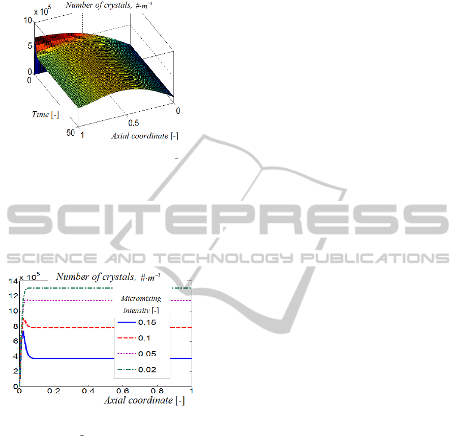
Figure 1: Time evolution of the axial distribution of popu-

lation density function of crystals for Pe=10 and

t .

tion rate as the state of mixing was increased along

the axial coordinate. At the same time, the number

of crystals is decreased due to crystal agglomeration.

Figure 2 shows the effects of micromixing in-

tensity on the steady state axial distribution of crys-

tals illustrating the strong influence of micromixing

on the number of crystals produced in the process.

Figure 2: Effects of micromixing intensity on the steady

state axial distribution of population density function of

crystals for Pe=10 and

1=t .

6 CONCLUSIONS

The population balance approach was applied to de-

velop a three-scale model for disperse systems using

the multi-scale methodology of complex systems. It

was shown that marking out the individual disperse

objects for microlevel of the system the population

balance equation, containing also terms describing

collision interchange of extensive quantities between

the disperse elements and motion in the physical

space is a meso-scale model. In this interpretation,

the macro-scale model is formulated by means of the

moments of internal quantities of disperse elements.

As an example, a two-population model, governing

the coupled behaviour of crystal and fluid element

populations is presented for describing micromixing

in reaction crystallization.

ACKNOWLEDGEMENTS

This work was supported by the Hungarian Scien-

tific Research Fund under Grant K 77955 which is

gratefully acknowledged.

REFERENCES

Gardiner, C. W., 1983. Handbook of Stochastic Methods

for Physics, Chemistry and the Natural Sciences.

Springer-Verlag, Berlin.

Eberard, D., Lefèvre, L., Maschke, B., 2005.

International

Conference on Physics and Control

, 543-547

Ingram, G. D., Cameron, I. T., 2002. Challenges in

multi-scale modeling and its application to granulation

sys-tems. Proceedings of APCChE 2002/Chemeca.

Lakatos, B. G., 2008. Population balance model for

mixing in continuous flow systems. Chemical

Engineering Science, 63 (2) 404-423.

Lakatos, B. G. 2010. Moment method for multidimen-

sional population balance models. Proceedings 4

In-

ternational Conference on Population Balance Mo-

delling, Berlin, pp. 885-903.

Lakatos, B. G., Bárkányi, Á., Németh, S., 2011. Con-

tinuous stirred tank coalescence/redispersion reactor:

A simulation study. Chemical Engineering Journal,

169, 247-257.

Li, J., Zhang, J., Ge, W., Liu, X., 2004. Multi-scale meth-

odology for complex systems. Chemical Engineering

Science, 59, 1687–1700.

Mazzotti, M., 2010. Multi-scale and multidimensional po-

pulation balance modelling. 4

International Confer-

ence on Population Balance Modelling, Keynote Lec-

ture. Berlin.

Sobczyk, K., 1991. Stochastic Differential Equations with

Applications to Physics and Engineering. Kluwer

Academic Publishers.

MULTI-SCALE APPROACH TO POPULATION BALANCE MODELLING OF DISPERSE SYSTEMS

191