AN HYBRID APPROACH TO FEATURE SELECTION FOR MIXED
CATEGORICAL AND CONTINUOUS DATA
Gauthier Doquire and Michel Verleysen
ICTEAM Institute, Machine Learning Group, Universit
´
e catholique de Louvain
pl. du Levant 3, 1348 Louvain-la-Neuve, Belgium
Keywords:
Feature selection, Categorical features, Continuous features, Mutual information.
Abstract:
This paper proposes an algorithm for feature selection in the case of mixed data. It consists in ranking inde-
pendently the categorical and the continuous features before recombining them according to the accuracy of
a classifier. The popular mutual information criterion is used in both ranking procedures. The proposed algo-
rithm thus avoids the use of any similarity measure between samples described by continuous and categorical
attributes, which can be unadapted to many real-world problems. It is able to effectively detect the most useful
features of each type and its effectiveness is experimentally demonstrated on four real-world data sets.
1 INTRODUCTION
Feature selection is a key problem in many machine
learning, pattern recognition or data mining applica-
tions. Indeed the ways to acquire and store data in-
crease every day. A lot of features are thus typically
gathered for a specific problem while many of them
can be either redundant or irrelevant. These useless
features often tend to decrease the performances of
the learning (classification or regression) algorithms
(Guyon and Elisseeff, 2003) and slower the whole
learning process. Moreover, reducing the number of
attributes leads to a better interpretability of the prob-
lem and of the models, which is of crucial importance
in many industrial and medical applications. Feature
selection thus plays a major role both from a learning
and from an application point of view.
Due to the importance of the problem, many fea-
ture selection algorithms have been proposed in the
past few years. However, the great majority of them
are designed to work only with continuous or cate-
gorical features and are thus not well suited to handle
data sets with both type of features, while mixed data
are encountered in many real-world situations. To il-
lustrate this, two examples are given. First, the results
of medical surveys can include continuous attributes
as the size or the blood pressure of a patient, together
with categorical ones as the sex or the presence or ab-
sence of a symptom. In another field, socio-economic
data can contain discrete variables about individuals
such as their kind of job or the city they come from,
as well as continuous ones like their income.
Algorithms dealing with continuous and discrete
attributes are thus needed. Two obvious ways to han-
dle problems with mixed attributes are turning the
problem into a categorical or a continuous one. Un-
fortunately, both approaches have strong drawbacks.
The first idea would consist in coding the categor-
ical attributes into discrete numerical values. It would
then be possible to compute distances between ob-
servations as if all features were continuous. How-
ever, this approach is not likely to work well. In-
deed, permuting the code for two categorical values
could lead to different values of distance. To cir-
cumvent this problem, Bar-Hen and Daudin (1995)
proposed to use a generalized Mahalanobis distance,
while Kononenko (1994) employs the Euclidean dis-
tance for continuous features and the Hamming dis-
tance for categorical ones. The second idea is to dis-
cretize continuous features before running an algo-
rithm designed for discrete data (Hall, 2000). Even
if appealing, this approach may lead to a loss of in-
formation and makes the feature selection efficiency
extremely dependant on the discretization technique.
Recently, Tang and Mao proposed a method based
on the error probability (Tang and Mao, 2007) while
Hu et al. reported very satisfactory results using rough
set models generalized to the mixed case (Hu et al.,
2008). In this last paper, the authors base their work
on neighborood relationships between mixed sam-
ples, defined in the following way. First, to be consid-
ered as neighbors, two samples must have the same
394
Doquire G. and Verleysen M..
AN HYBRID APPROACH TO FEATURE SELECTION FOR MIXED CATEGORICAL AND CONTINUOUS DATA.
DOI: 10.5220/0003634903860393
In Proceedings of the International Conference on Knowledge Discovery and Information Retrieval (KDIR-2011), pages 386-393
ISBN: 978-989-8425-79-9
Copyright
c
 2011 SCITEPRESS (Science and Technology Publications, Lda.)

values for all their discrete attributes. Then, depend-
ing on the approach chosen and according to the con-
tinuous features, the Euclidean distance between the
samples has to be below a fixed treshold or one of
the sample has to belong to the k nearest neighbors of
the other. The method thus makes a strong hypoth-
esis about the notion of proximity between samples,
which can be totally inconsistent with some problems
as will be illustrated later in this work.
In contrast, the approach proposed in this paper
does not consider any notion of relationship between
mixed samples. Instead, the objective is to correctly
detect the most useful features of each kind and to
combine them to optimize the performance of predic-
tion models. More precisely, the features of each type
are first ranked independently; two independent lists
are produced. The lists are then combined accord-
ing to the accuracy of a classifier. Mutual information
(MI) based feature selection is employed for the rank-
ing of both continuous and categorical features.
The rest of the paper is organized as follows. Sec-
tion 2 briefly recalls basic notions about MI. The pro-
posed methodology is described in Section 3 and ex-
perimental results are given in Section 4. Conclusions
are drawn in Section 5 which also contains some fu-
ture work perspectives.
2 MUTUAL INFORMATION
In this section, basic concepts about MI are intro-
duced and a few words are given about its estimation.
2.1 Definitions
MI (Shannon, 1948) is a criterion from the informa-
tion theory which has proven to be very efficient in
feature selection (Battiti, 1994; Fleuret, 2004) mainly
because it is able to detect non linear relationships
between variables, while other popular criteria as the
well-known correlation coefficient are limited to lin-
ear relationships. Moreover, MI can handle groups of
vectors, i.e. multidimensional variables.
MI is intuitively a symmetric measure of the in-
formation two random variables X and Y carry about
each other and is formally defined as follows:
I(X;Y ) = H(X ) + H(Y )−H(X,Y ) (1)
where H(X ) is the entropy of X:
H(X ) = −
Z
f
X
(x)log f
X
(x) dx (2)
with f
X
being the probability density function (pdf) of
X. H(X,Y ) is the entropy of the joint variable (X,Y )
defined in the same way.
The MI can be reformulated as:
I(X;Y ) =
Z Z
f
X,Y
(x,y) log
f
X,Y
(x,y)
f
X
(x) f
Y
(y)
dx dy. (3)
This last equation defines MI as the Kullback-Leibler
divergence between the joint distribution f
X,Y
and the
product of the distributions f
X
and f
Y
, these quanti-
tites being equal for independant variables.
As in practice none of the pdf f
X
, f
Y
and f
X,Y
are
known, MI can not be computed analytically but has
to be estimated from the data set.
2.2 MI Estimation
Traditional MI estimators are based on histograms or
kernels (Parzen, 1962) density estimators which are
used to approximate the value of the MI according for
example to (1) (Kwak and Choi, 2002). Despites its
popularity, this approach has the huge drawback that
it is unreliable for high-dimensional data. Indeed, as
the dimension of the space increases, if the number of
available samples remains constant, these points will
not be sufficient to sample the space with an accept-
able resolution. For histograms, most of the boxes
will be empty and the estimates are likely to be in-
accurate. Things will not be different for kernel es-
timators which are essentially smoothed histograms.
These problems are a direct consequence of the curse
of dimensionality (Bellman, 1961; Verleysen, 2003),
stating that the number of points needed to sample
a space at a given resolution increases exponentially
with the dimension of the space; if p points are needed
to sample a one-dimensional space at a given resolu-
tion, p
n
points will be needed if the dimension is n.
Since in this paper MI estimation is needed for
multi-dimensional data points, other estimators have
to be considered. To this end, a recently introduced
family of estimators based on the principle of near-
est neighbors are used (Kraskov et al., 2004; G
´
omez-
Verdejo et al., 2009). These estimators have the ad-
vantage that they do not estimate the entropy directly
and are thus expected to be more robust if the di-
mension of the space increases. They are inspired
by the Kozachenko-Leonenko estimator of entropy
(Kozachenko and Leonenko, 1987):
ˆ
H(X) = −ψ(k) + ψ(N) + log(c
d
) +
d
n
N
∑
n=1
log(ε
X
(n,k))
(4)
where k is the number of nearest neighbors consid-
ered, N the number of samples of a random variable
X, d the dimensionality of these samples, c
d
the vol-
ume of a unitary ball of dimension d and ε
X
(n,k)
twice the distance from the n
th
observation in X to
AN HYBRID APPROACH TO FEATURE SELECTION FOR MIXED CATEGORICAL AND CONTINUOUS DATA
395

its k
th
nearest neighbor; ψ is the digamma function:
ψ(k) =
Γ
0
(k)
Γ(k)
=
d
dk
lnΓ(k) , Γ(k) =
Z
∞
0
x
k−1
e
−x
dx.
Using (4), Kraskov et al. (Kraskov et al., 2004) de-
rived two slightly different estimators for regression
problems (i.e. for problems with a continuous out-
put). The most widely used one is:
ˆ
I(X;Y ) =ψ(N) + ψ(K) −
1
k
−
1
N
N
∑
n=1
(ψ(τ
x
(n)) + ψ(τ
y
(n)))
(5)
where τ
x
(n) is the number of points located no further
than ε
X
(n,k) from the n
th
observation in the X space;
τ
y
(n) is defined similarly in the Y space with ε
Y
(n,k).
In case of a classification problem, Y is a dis-
crete vector representing the class labels. Calling L
the number of classes, Gomez et al. (G
´
omez-Verdejo
et al., 2009) took into account the fact that the prob-
ability distribution of Y is estimated by p(y = y
l
) =
n
l
/N, where n
l
is the number of points whose class
value is y
l
, and proposed to estimate the MI as:
ˆ
I
cat
(X;Y ) = ψ(N) −
1
N
n
l
ψ(n
l
)+
d
N
"
N
∑
n=1
log(ε
X
(n,K)) −
L
∑
l=1
∑
n∈y
l
log(ε
l
(n,K))
#
.
(6)
In this last equation, ε
l
(n,K) is defined in the same
way as ε
X
(n,K) in (4) but the neighbors are limited to
the points having the class label y
l
.
If both X and Y are categorical features, equations
(2) and (3) become sums where the probabilities can
be estimated from the samples in the learning set by
simple counting and no estimator is needed. Assume
X (resp. Y ) takes s
x
(s
y
) different values x
1
.. .x
s
x
(y
1
.. .y
s
y
), each with a probability p
x
i
(p
y
i
) and de-
note by p
x
i
,y
i
the joint probability of x
i
and y
i
, then:
I(X;Y ) =
s
x
∑
i=1
s
y
∑
j=1
p
x
i
,y
j
log
p
x
i
,y
j
p
x
i
p
y
j
. (7)
3 METHODOLOGY
This section presents the proposed feature selection
procedure. It ends with a few comments on the filter /
wrapper dilemma.
3.1 Lists Ranking
As already discussed, this paper suggests avoiding the
use of any similarity measure between mixed data
points. To this end, the proposed procedure starts
by separating the continuous and the categorical fea-
tures. Both groups of features are then ranked inde-
pendently, according to the following strategies.
3.1.1 Continuous Features
For continuous features, the multivariate MI criterion
is considered, meaning that the MI is directly esti-
mated between a set X of features and the output Y .
The nearest neighbors based MI estimators
(Kraskov et al., 2004; G
´
omez-Verdejo et al., 2009)
described previously are particularly well suited for
multivariate MI estimation. Indeed, as already ex-
plained, they do not require the estimation of multi-
variate probability density functions. This crucial ad-
vantage allows us to evaluate robustly the MI between
groups of features with a limited number of samples.
As an example the estimator described in (Kraskov
et al., 2004) has been used sucessfully in feature se-
lection for regression problems (Rossi et al., 2006).
In this paper, the multivariate MI estimator is com-
bined with a greedy forward search procedure; at each
step of the selection procedure, the feature whose ad-
dition to the set of already selected features leads to
the largest multivariate MI with the output is selected.
This choice is never questioned again, hence the name
forward. Algorithm 1 illustrates a greedy forward
search procedure for a relevance criterion c to be max-
imized, with R{i} being the i
th
element of R.
Obviously, in such a procedure, the possible re-
dundancy between the features is implicitely taken
into account since the selection of a feature carrying
no more information about the output than the already
selected ones will result in no increase of the MI.
3.1.2 Categorical Features
It is important to note that the multivariate MI esti-
mators (Kraskov et al., 2004; G
´
omez-Verdejo et al.,
2009) should not be considered for categorical fea-
tures. Indeed, for categorical data it is likely that
the distances between a sample and several others are
identical, especially in the first steps of the forward
selection procedure. These ex-aequos could bring
confusion in the determination of the nearest neigh-
bors and harm the MI estimation. Moreover, using di-
rectly equation (7) can be untractable in practice. As
an example, if X consists of 20 features, each taking 3
possible discrete values, the total number of possible
values s
x
for points in X is 3
20
> 3 × 10
9
.
KDIR 2011 - International Conference on Knowledge Discovery and Information Retrieval
396

Another criterion than multivariate MI has thus to
be thought of. In this paper, the minimal-Redundancy
maximal-Relevance (mRmR) principle is used since
it has proven to be very efficient in feature selection
when combined with the MI criterion (Peng et al.,
2005). The idea is to select a set of maximally in-
formative but not redundant features.
This principle is also combined with a greedy for-
ward search strategy: suppose a subset of features
has already been selected; one searches for the uns-
elected feature which maximises D − R where D, the
estimated relevance, is the MI between the new fea-
ture and the output. R is the estimated redundancy
and can be measured by the average MI between the
new feature and each of the already selected features.
Denote by S the set of indices of already selected fea-
tures; the mRmR criterion D − R for feature i (i /∈ S)
given an output vector Y is:
mRmR( f
i
) = I( f
i
;Y ) −
1
|S|
∑
j∈S
I( f
i
; f
j
). (8)
All MI estimations or computations in the mRmR
procedure are thus bivariate (i.e. involve only two
variables). Of course, bivariate methods are not ex-
pected to perform as well as multivariate ones since
they only consider pairwise redundancy or relevance.
A simple example showing this is the well-known
XOR problem. It consists of two random binary vec-
tors X
1
, X
2
and an output Y whose i
th
element is 1 if
the i
th
elements of X
1
and X
2
are different and 0 other-
wise. Individually, both vectors carry no information
about the output Y . However, together they entirely
determine it. Thus, even if X
1
is selected, a mRmR
procedure will not be able to determine X
2
as relevant
while a multivariate approach will.
3.2 Combination of the Lists
Once established, the two lists are combined accord-
ing to the accuracy (the percentage of well-classified
samples) of a classification model. First, the accura-
cies of a model built on the first continuous or the first
categorical feature are compared. The feature leading
to the best result is chosen and removed from the list
it belongs to. The selected feature is then combined
with the best continuous or with the best categorical
feature that still belong to their respective lists, i.e.
that has not been selected yet; the subset for which
a model performs the best is selected, and so on un-
til all features have been selected. The whole feature
selection procedure is described in Algorithm 2.
Input: A set F of features i, i = 1 : n
f
A class labels vector Y
Output: A list L of sorted indices of features.
begin
R ←− 1 : n
f
//R is the set of indices of not yet
selected features
L ←−
/
0
for k = 1 : n
f
do
foreach i ∈ R do
set ←− L ∪ R
{
i
}
score
{
i
}
←− c(set,Y )
end
winner ←− argmax
j
score
{
j
}
L ←− [L; R
{
winner
}
]
R ←− R \R
{
winner
}
clear score
end
end
Algorithm 1: Forward search procedure to maximize a cri-
terion c.
3.3 Filter or Wrapper Feature Selection
As can be seen from the previous developments, two
different approaches to feature selection are succes-
sively used to produce a global algorithm. First,
building the two lists is made by using filter methods.
This means that no classification model is used and
that the selection is rather based on a relevance crite-
rion, such as MI in this paper. On the other hand, the
combination of the lists does require a specific classi-
fier and is thus a wrapper procedure.
Wrappers are generally expected to lead to better
results than filters since they are designed to optimize
the performances of a specific classifier. Of course,
wrappers are also usually much slower than filters,
precisely because of the fact they have to build a huge
number of classification models with possible hyper-
parameters to tune.
As an example, the exhaustive wrapper approach
consisting in testing all the possible feature subsets
would require building 2
n
f
models, n
f
being the num-
ber of features. If there are 20 features, about 10
6
classifiers must be built. This method thus becomes
quickly untractable as the number of features grows.
An alternative is to use heuristics such as the greedy
forward search presented in Algorithm 1. The num-
ber of models to build is then
n
f
(n
f
+1)
2
− 1 which is
still unrealistic for complex models.
On the contrary, the approach proposed in this pa-
per only requires the construction of at most n
f
− 1
classifiers. Indeed, Algorithm 2 emphasizes the fact
that the use of a classification model is needed only
if none of the lists are empty; in practice the num-
ber of models to build will thus often be smaller than
AN HYBRID APPROACH TO FEATURE SELECTION FOR MIXED CATEGORICAL AND CONTINUOUS DATA
397

n
f
− 1. In addition
n
cont
(n
cont
+1)
2
+
n
cat
(n
cat
+1)
2
− 2 eval-
uations of the MI are necessary, n
cat
and n
cont
being
respectively the number of categorical and continuous
features. A compromise between both approaches is
thus found, which prevents us to use any similarity
measure between mixed samples, while keeping the
computional burden of the procedure relatively low.
Input: A set of categorical features F
cat
{
i
}
,
i = 1 : n
cat
A set of continuous features F
cont
{
i
}
,
i = 1 : n
cont
A class labels vector Y.
Output: A list L of sorted indices of features.
begin
InCat ←− SortCat(F
cat
,Y )
//Get the sorted list of indices for
categorical features
InCon ←− SortCon(F
cont
,Y )
//Get the sorted list of indices for
continuous features
L ←−
/
0
for k = 1 : n
cat
+ n
cont
do
if InCat 6=
/
0 and InCon 6=
/
0 then
AccCat ←− Acc(L ∪InCat
{
1
}
,Y )
AccCon ←− Acc(L ∪ InCon
{
1
}
,Y )
//Function Acc(.) gives the
accuracy of a classifier.
if AccCat < AccCon then
L ←− L ∪ InCon
{
1
}
delete InCon
{
1
}
else
L ←− L ∪ InCat
{
1
}
delete InCat
{
1
}
end
else
if InCat =
/
0 then
L ←− L ∪ InCon
{
1
}
delete InCon
{
1
}
else
L ←− L ∪ InCat
{
1
}
delete InCat
{
1
}
end
end
end
end
Algorithm 2: Proposed feature selection algorithm.
4 EXPERIMENTAL RESULTS
To assess the performance of the proposed feature se-
lection algorithms, experiments are conducted on ar-
tificial and real-world data sets. The limitations of
methods based on a given similarity measure between
mixed samples are first emphasized on a very simple
Table 1: Description of the datasests used in the experi-
ments.
Name samples cont. features cat. features classes
Heart 270 6 7 2
Hepatitis 80 6 13 2
Australian Credit 690 6 8 2
Contraception 1473 2 7 3
toy problem. Results obtained on four UCI (Asuncion
and Newman, 2007) data sets then confirm the inter-
est of the proposed approach.
Two classification models are used in this study.
The first one is a Naive Bayes classifier with probabil-
ities for continuous attributes estimated using Parzen
window density estimation (Parzen, 1962) and those
for categorical attributes estimated by counting.
The second one is a 5-nearest neighbors classifier,
with distances between samples computed by the Het-
erogeneous Euclidean-Overlap Metric (HEOM) (Wil-
son and Martinez, 1997) while other choices could
as well have been made (see e.g. (Boriah et al.,
2008)). This metric uses different distance functions
for categorical and continuous attributes. It is defined
for two vectors X = [X
1
.. .X
m
] and Y = [Y
1
.. .Y
m
] as
d
heom
(X,Y ) =
p
∑
m
a=1
d
a
(X
a
,Y
a
)
2
where
d
a
(x,y) :=
(
overlap(x,y) if a is categorial
|
x−y
|
max
a
−min
a
if a is continuous
with max
a
and min
a
, respectively the maximal and
minimal values observed for the a
th
feature in the
training set, and overlap(x,y) = 1 − δ(x,y) (δ denot-
ing the Kronecker delta, δ(x,y) = 1 if x = y and 0
otherwise). These models have mainly been chosen
because they are both known to suffer dramatically
from the presence of irrelevant features in compari-
son with, for example, decision trees.
In this section, we compare the proposed feature
selection approach with the algorithm by Hu and al.
(Hu et al., 2008). As already explained, in that paper,
the authors consider two points as neighbors if their
categorical attributes are equal and if one is among
the k nearest neighbors of the other or if the distance
between them is not too large according to their nu-
merical attributes (there are thus two versions of the
algorithm). Then, they look for the features for which
the largest number of points share their class label
with at least a given fraction of their neighbors. The
methodology is thus extremely dependent on the cho-
sen definition of neighborhood. Even if this definition
can be modified, it is not easy, given an unknown data
set, to determine a priori which relation can be a good
choice. Among the two versions of Hu and al.’s al-
gorithm, only the nearest neighbors-based one will be
considered in this work, since it has been shown more
KDIR 2011 - International Conference on Knowledge Discovery and Information Retrieval
398

efficient in practice (Hu et al., 2008), which was con-
firmed by our experiments.
4.1 Toy Problem
To underline the aformentionned drawbacks, a toy
problem is considered to show the limitations of
methods based on dissimilarities for mixed data.
It consists in a data set X containing two categori-
cal variables (X
1
,X
2
) taking two possible discrete val-
ues with equal probability and two continuous vari-
ables (X
3
,X
4
) uniformly distributed over [0; 1]. The
sample size is 100. A class labels vector Y is also
built from X ; the points whose value of X
3
is below
0.15 or above 0.85 are given the class label 1 and the
other points are given the class label −1. The only
relevant variable is thus X
3
, which sould be selected
in first place by accurate feature selection algorithms.
However, the problem with Hu et al.’s method is
that many points with class label 1 do not have enough
neighbors with the same label. Feature X
3
will not
thus be detected as relevant by the algorithms. More
precisely, over 50 repetitions, X
3
has been selected in
the first place only in 28 cases. With the approach
proposed in this paper, X
3
has been selected first in
the 50 repetitions of the experiment.
Interestingly, if the problem is modified such that
points for which the value of X
3
is between 0.4 and
0.7 have class label 1 and other points have class label
−1, then Hu and al.’s algorithm always detect X
3
has
the most relevant variable. Although the proportion
of both classes in the two problems are the same, the
second one is more compatible with the chosen def-
inition of neighborhood, explaining the better results
obtained. Of course, this definition of neighborhood
could be modified to better fit the first problem but
would then likely be inaccurate in other situations.
4.2 Real-world Data Sets
Four classification benchmark data sets from the UCI
Machine Learning Repository (Asuncion and New-
man, 2007) are used in the study to further illustrate
the interest of the proposed approach. All contain
continuous and categorical attributes and are summa-
rized in Table 1. Two come from the medical world,
one is concerned with whether an applicant should re-
ceive a credit card or not and the last one is about the
choice of a contraceptive method. The data sets used
in this work are not the same as those considered in
(Hu et al., 2008) since many of the latest do not actu-
ally contain mixed features.
As a preprocessing, observations containing miss-
ing values are deleted. Moreover, continuous at-
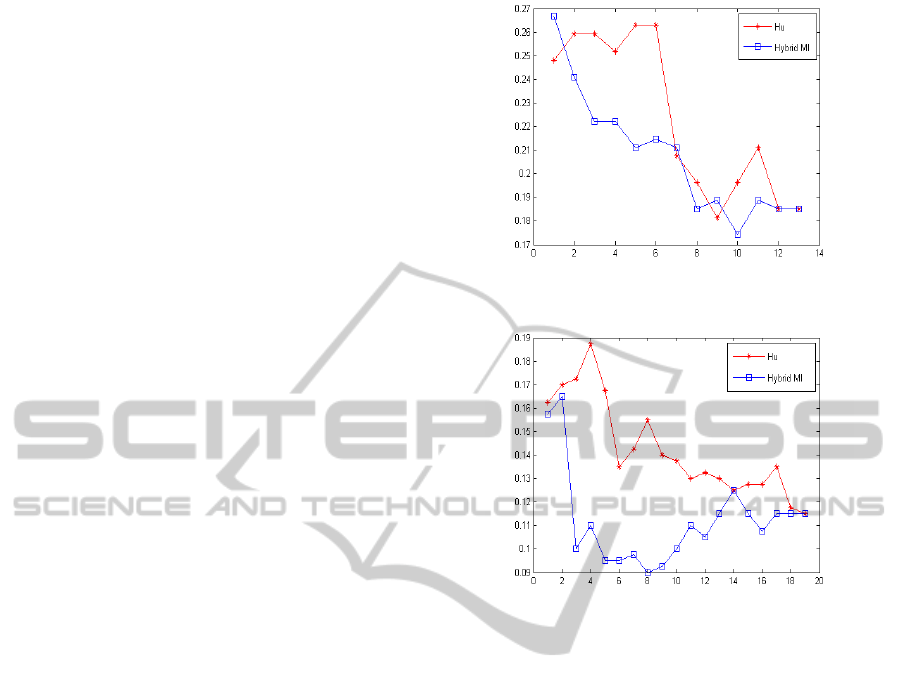
Figure 1: Error rate as a function of the number of selected
features: Heart data set and naive Bayes classifier.
Figure 2: Error rate as a function of the number of selected
features: Hepatitis data set and naive Bayes classifier.
tributes are normalized by removing their mean and
dividing them by their standard deviation in order
to make the contribution of each attribute to the Eu-
clidean distance equivalent in the MI estimation. As
suggested in (G
´
omez-Verdejo et al., 2009), for con-
tinuous features, the MI is estimated over a range of
different values of the parameter k and then averaged
to prevent strong underfitting or overfitting. In this
paper, 4 to 12 neighbors are considered except for the
Hepatitis data set for which 4 to 6 neighbors are taken
into account. This is due to the fact that a class is
represented by only a few samples in this data set.
The criterion of comparison is the classification
error rate. It is estimated through a 5-fold cross vali-
dation procedure repeated 5 times with different ran-
dom shufflings of the data set. The presented error
rates are obtained on the test set, independant of the
training set used to train the classifier. The feature to
choose at each wrapper step is determined by a 5-fold
cross validation on the training set.
Figures 1 to 7 show the average classification er-
ror rate achieved by the proposed method (referred to
as Hybrid MI) and by Hu and al.’s one with respect to
the number of features selected. As can be seen, the
approach is very competitive with both classifiers and
leads to the global smallest misclassification rate in 7
AN HYBRID APPROACH TO FEATURE SELECTION FOR MIXED CATEGORICAL AND CONTINUOUS DATA
399

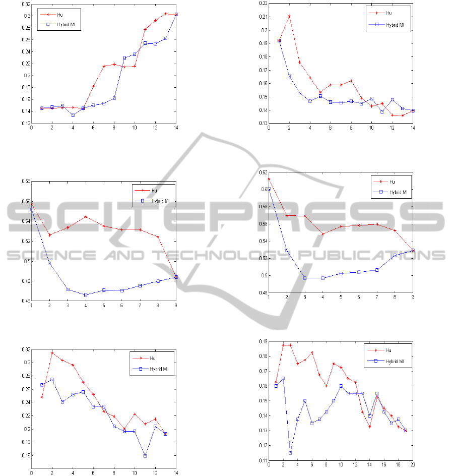
Figure 3: Error rate as a function of the number of selected
features: Australian credit data set and naive Bayes classi-
fier.
Figure 4: Error rate as a function of the number of selected
features: Contraception data set and naive Bayes classifier.
Figure 5: Error rate as a function of the number of selected
features: Heart data set and k-nn classifier.
of the 8 experiments. Moreover, for the Hepatitis and
the Contraception data sets, it is the only approach
selecting a subset of features leading to better perfor-
mances than the set of all features. The improvement
in classification accuracy is thus obvious.
5 CONCLUSIONS
This paper introduces a new feature selection method-
Figure 6: Error rate as a function of the number of selected
features: Australian credit data set and k-nn classifier.
Figure 7: Error rate as a function of the number of selected
features: Contraception data set and k-nn classifier.
Figure 8: Error rate as a function of the number of selected
features: Hepatitis data set and k-nn classifier.
ology for mixed data, i.e. for data with both categori-
cal and continuous attributes. The idea of the method
is to independently rank both types of features before
recombining them guided by the accuracy of a clas-
sifier. The proposed algorithm is thus a combination
of a filter and a wrapper approach to feature selec-
tion. The well-known MI criterion is used to produce
both ranked lists. For continuous features, multidi-
mensional MI estimation is used while a mRmR ap-
proach is considered for categorical features.
One of the most problematic issues for feature se-
KDIR 2011 - International Conference on Knowledge Discovery and Information Retrieval
400

lection algorithms dealing with mixed data is to chose
an appropriate relationship between categorical and
continuous features leading to a sound similarity mea-
sure or neighborood definition between observations.
This new method simply alleviates this problem by
ignoring this unknown relationship. The hope is to
compensate the loss of information induced by this
hypothesis by a more accurate ranking of features of
each type and by the use of a classification model.
Even if the approach requires the explicit building
of prediction models, the number of models to build
is small compared to a pure wrapper approach. More-
over, experimental results on four data sets show the
interest in terms of the accuracy of two classifiers.
All the developments presented in this paper could
be applied to regression problems (problems with a
continuous output); the only modifications needed
would be to use the MI estimator (5) instead of (6)
for the continuous features and the mRmR approach
for the categorical ones. It would thus be interesting
to test the proposed approach on such problems.
REFERENCES
Asuncion, A. and Newman, D. (2007). UCI machine learn-
ing repository. University of California, Irvine, School
of Information and Computer Sciences, available at
http://www.ics.uci.edu/∼mlearn/MLRepository.html.
Battiti, R. (1994). Using mutual information for select-
ing features in supervised neural net learning. IEEE
Transactions on Neural Networks, 5:537–550.
Bellman, R. (1961). Adaptive Control Processes: A Guided
Tour. Princeton University Press.
Boriah, S., Chandola, V., and Kumar, V. (2008). Similarity
measures for categorical data: A comparative evalua-
tion. In SDM’08, pages 243–254.
Fleuret, F. (2004). Fast binary feature selection with con-
ditional mutual information. J. Mach. Learn. Res.,
5:1531–1555.
G
´
omez-Verdejo, V., Verleysen, M., and Fleury, J. (2009).
Information-theoretic feature selection for functional
data classification. Neurocomputing, 72:3580–3589.
Guyon, I. and Elisseeff, A. (2003). An introduction to
variable and feature selection. J. Mach. Learn. Res.,
3:1157–1182.
Hall, M. A. (2000). Correlation-based feature selection
for discrete and numeric class machine learning. In
Proceedings of ICML 2000, pages 359–366. Morgan
Kaufmann Publishers Inc.
Hu, Q., Liu, J., and Yu, D. (2008). Mixed feature selec-
tion based on granulation and approximation. Know.-
Based Syst., 21:294–304.
Kozachenko, L. F. and Leonenko, N. (1987). Sample es-
timate of the entropy of a random vector. Problems
Inform. Transmission, 23:95–101.
Kraskov, A., St
¨
ogbauer, H., and Grassberger, P. (2004). Es-
timating mutual information. Physical review. E, Sta-
tistical, nonlinear, and soft matter physics, 69(6 Pt 2).
Kwak, N. and Choi, C.-H. (2002). Input feature selection
by mutual information based on parzen window. IEEE
Trans. Pattern Anal. Mach. Intell., 24:1667–1671.
Parzen, E. (1962). On the estimation of a probability density
function and mode. Annals of Mathematical Statistics,
33:1065–1076.
Peng, H., Long, F., and Ding, C. (2005). Fea-
ture selection based on mutual information: Cri-
teria of max-dependency, max-relevance and min-
redundancy. IEEE Trans. Pattern Anal. Mach. Intell.,
27:1226–1238.
Rossi, F., Lendasse, A., Franc¸ois, D., Wertz, V., and Verley-
sen, M. (2006). Mutual information for the selection
of relevant variables in spectrometric nonlinear mod-
elling. Chemometrics and Intelligent Laboratory Sys-
tems, 80(2):215–226.
Shannon, C. E. (1948). A mathematical theory of commu-
nication. The Bell system technical journal, 27:379–
423.
Tang, W. and Mao, K. Z. (2007). Feature selection algo-
rithm for mixed data with both nominal and continu-
ous features. Pattern Recogn. Lett., 28:563–571.
Verleysen, M. (2003). Learning high-dimensional data.
Limitations and Future Trends in Neural Computa-
tion, 186:141–162.
Wilson, D. R. and Martinez, T. R. (1997). Improved hetero-
geneous distance functions. J. Artif. Int. Res., 6:1–34.
AN HYBRID APPROACH TO FEATURE SELECTION FOR MIXED CATEGORICAL AND CONTINUOUS DATA
401