
A MEMETIC ALGORITHM FOR A CONTINUOUS CASE OF THE
BERTH ALLOCATION PROBLEM
Geraldo Regis Mauri
1
, Larice Nogueira de Andrade
2
and Luiz Antonio Nogueira Lorena
3
1
Federal University of Esp´ırito Santo - UFES, Alegre, ES, Brazil
2
Federal University of Triˆangulo Mineiro - UFTM, Uberaba, MG, Brazil
3
National Institute for Space Research - INPE, S˜ao Jos´e dos Campos, SP, Brazil
Keywords:
Berth allocation, Memetic algorithm, Simulated annealing, Combinatorial optimization.
Abstract:
This work presents a Memetic Algorithm heuristic to solve a continuous case of the Berth Allocation Problem
(BAP). The BAP deals with programming and allocating ships to berthing areas along a quay. In general, the
continuous case considers that ships have different lengths and can moor anywhere along the quay. However,
we consider a quay divided in berths that have limited areas and different equipments to handle the ships. So,
we must to assign the ships to berths and determine the berthing time and position for each ship. We treat
the ships as rectangles to be placed into a space × time area avoiding overlaps and satisfying time window
constraints. Our MA uses a Simulated Annealing (SA) as the local search mechanism, and SA is also applied
in a stand alone way to solve the BAP. A two-phase heuristic is also presented to compute the berthing time
and position for all of ships during MA and SA execution. Computational results are performed on a set of
instances proposed in the literature and new best-known solutions are presented.
1 INTRODUCTION
The port importance grows with the increasing
progress in the construction technology of great ships.
Besides, due to the improved trades among the na-
tions caused by globalization, the frequency of trans-
ports among ports also increases, mainly due to the
constant economical growth and volume of the trade
among several countries.
Maritime transport can be seen as a central pil-
lar for the international trade. Approximately 80% of
global market is conducted through the sea (Buhrkal
et al., 2011). Moreover, in 2008 the fleet of ships car-
rying containers had an increase in capacity of 17.3
million tons, or 11.9%, and now represents 13.6% of
world total. In 2009, the world merchant fleet reached
1.19 million, an increase of 6.7% compared to Jan-
uary 2008, and since the beginning of the decade, the
number of containers increased by 154% (UNCTAD,
2009).
Due to intense flow of ships and containers in
ports, these are forced to invest heavily to accommo-
date the ships, deepening and widening channels and
building new installations of moor, everything to min-
imize the service time of the ships. So, a port should
operates in an efficient way (Hansen et al., 2008).
The allocation and programming of ships to berths
have a primary impact on the efficiency of these op-
erations (Imai et al., 2003). Vis and Koster (2003)
present a discussion about the decision problems that
appear in a port. A classification of the processes and
operations of different marine terminals is presented
by Steenken et al. (2004). The crucial problem in a
port administration is optimizing the balance among
the ships holder that demand fast services, and the
economical use of the available resources into the port
(Dragovic et al., 2005).
The Berth Allocation Problem (BAP) consists of
optimally assigning ships to berthing areas along a
quay in a port. The choice of “where” and “when”
the ships shall berth is the main decision to be made
in that process (Cordeau et al., 2005).
The BAP has a lot of physical and technical re-
strictions, among others. This makes possible to
model it in different ways. Considering the spatial
aspects of the berths, the BAP can be modeled as dis-
crete and continuous (Imai et al., 2005). In the dis-
crete case, the quay is divided into several berths and
only one ship is serviced at a time in every berth, re-
gardless of their length. In the continuous case, there
is no division of the quay and thus the ships can moor
at any position. Another conception for the continu-
105
Regis Mauri G., Nogueira de Andrade L. and Antonio Nogueira Lorena L..
A MEMETIC ALGORITHM FOR A CONTINUOUS CASE OF THE BERTH ALLOCATION PROBLEM.
DOI: 10.5220/0003636601050113
In Proceedings of the International Conference on Evolutionary Computation Theory and Applications (ECTA-2011), pages 105-113
ISBN: 978-989-8425-83-6
Copyright
c
2011 SCITEPRESS (Science and Technology Publications, Lda.)

ous case considers that the quay is divided in berths,
but the big ships can occupy more than one posi-
tion, thus allowing small ships to share their berth
(Cordeau et al., 2005). This last approach represents
the real cases of a more appropriate way, where some
berths have different equipments (reaching limited ar-
eas) to operate specific type of cargo(container of var-
ious sizes, for example).
If we consider the arrival of ships, the BAP can be
still treated as static or dynamic (Imai et al., 2001).
The static case assumes all ships already in port for
the service, while the dynamic case allows ships to
arrive at any time (estimated in advance). In recent
works, we have notice that the term “dynamic” has
been unusual, because in practice, the static case is
not close to real situations. Then, the remainder of
this paper will denotes the “dynamic and continuous
case” only as continuous case.
This paper solves a continuous case of the BAP by
means of an effective Memetic Algorithm (MA) using
a Simulated Annealing (SA) as the local search mech-
anism. SA is also applied in a stand alone way, and
both SA and MA use a two-phase heuristic to com-
pute the berthing time and position for all of ships
presenting results that outperform those obtained by
another heuristic approach reported in the literature.
The remainder of this paper is organized as fol-
lows. The next section reports a brief literature re-
view. Section 3 presents details about the BAP. Our
MA, SA and two-phase heuristic are described in Sec-
tion 4. Computational results are presented in Section
5, followed by conclusions in Section 6.
2 BRIEF LITERATURE REVIEW
Initial works about the BAP appear at the end of the
80s, but these works have been gaining focus in the
last 10 years.
Approaches based on using heuristic alternatives
to solve the BAP are the most explored, and we be-
lieve that such methods have been predominating for
allowing the inclusion of several constraints in a “soft
way”.
Imai et al. (2001) present a method based on La-
grangian relaxation of the original problem. Two
years later, Imai et al. (2003) upgraded their approach
considering different service priorities between the
ships. Furthermore, the authors proposed a Genetic
Algorithm as a method of solution. The same authors
also treated a continuous case (see Imai et al. (2005)).
Cordeau et al. (2005) present a Tabu Search based
heuristic for solve two different models for a discrete
case of the BAP. They also present a TS heuristic for
a continuous case of the problem. They compared
their TS with a truncated branch-and-bound applied
to an exact formulation. Comparisons were made for
the discrete case. For the continuous approach, the
TS was able to solving more realistic instances than
those previously considered by other authors. The
proposed TS could handles various features of real-
life problems, including time windows and favorite
and acceptable berthing areas. The objective function
treated a weighted sum of the ship’s service times.
Mauri et al. (2008a) proposed an approach based
on the application of Simulated Annealing for solving
the discrete case of BAP. The authors treat the prob-
lem as a Multi-Depot Vehicle Routing Problem with
Time Windows (MDVRPTW). The computational re-
sults improved those obtained by CPLEX and Tabu
Search proposedby Cordeau et al. (2005). Mauri et al.
(2008b) solves the discrete case of the BAP by using a
hybrid method called PTA/LP, which uses the Popula-
tion Training Algorithm with a Linear Programming
model through a Column Generation technique. The
results improved those shown in their previous work.
Giallombardo et al. (2010) present two models
based on quadratic and linear programming to repre-
sent a discrete case of the BAP. Moreover, the authors
use a Tabu Search and a mathematical programming
technique to solve instances based on real data.
Recently, Buhrkal et al. (2011) reviewed some ap-
proaches about BAP and described three models for
the discrete berth allocation problem. The authors
proven the optimal solutions for some instances pre-
sented by Cordeau et al. (2005) for the discrete case
of BAP.
3 BERTH ALLOCATION
As mentioned before, the Berth Allocation Prob-
lem (BAP) consists of optimally assigning ships to
berthing areas along a quay in a port respecting sev-
eral physical and technical restrictions.
Related to the berth position, there exist con-
straints concerning to the depth of the water (allow-
able draft) and to the maximum distance from the
most favorable location along the quay, considering
the ship’s length and the location of the outbound and
inbound containers.
Some ports have hard allowable draft constraints
since they are located in geographical regions subject
to meaningful tide variation. In such cases, the ships
only can berth in known time windows of about two
hours around the high tide.
Besides this time window constraint, there exist
the time windows for completion time of ship servic-
ECTA 2011 - International Conference on Evolutionary Computation Theory and Applications
106
ing (Cordeau et al., 2005). The handling time of a
ship depends on its berthing point and it is a function
of the distance from the berth to the pick-up and de-
livery area of containers stored in the port yard. This
dependency strongly affects the performance of the
port (Cordeau et al., 2005).
Managers want to minimize both port and user
costs, which are related to service time. The objec-
tive of the BAP is usually to minimize the total ser-
vice time of all ships. Since ships do not have equal
importance, a weighted sum of the ship service times
may better reflect the management practice of some
ports. The weights in this sum can represent a pric-
ing scheme (demurrage) over delayed operations, the
number of container moves, and the urgent need of a
given load. Penalty terms can be explicitly included
in the objective function, for example, the demurrage
cost when the service time of a ship exceeds the con-
tracted value (see Barros et al. (2011), for example).
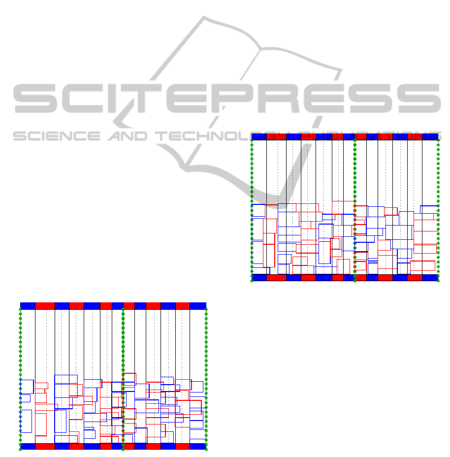
As reported by Cordeau et al. (2005), the BAP
can be represented in a two-dimensional area (see
Figures 1 and 2) considering the ships as rectangles
whose dimensions are length, including a safety mar-
gin, and handling time (space x time area). So, the
BAP can be defined by placing these rectangles in the
port area without overlapping and satisfying several
constraints.
The spatial dimension is ignored in the discrete
case of the BAP, and the berths can be described as
fixed length segments, or simple points. For the con-
tinuous case, we consider that the quay is also divided
in berths (as explained in Section 1), but now the spa-
tial dimension is not ignored. We will denote these
approaches as BAP-D and BAP-C, respectively. For
the BAP-C, a ship may occupy part of neighboring
berths (see Cordeau et al. (2005)).
0
50
100
150
200
250
300
SPACE
TIME
B1
B1
B2
B2
B3
B3
B4
B4
B5
B5
B6
B6
B7
B7
B8
B8
B9
B9
B10
B10
B11
B11
B12
B12
B13
B13
Figure 1: Optimal solution for BAP-D: i01 = 1409.
Cordeau et al. (2005) considered a quay divided
into berths with two parts, left and right. So, each
berth k has two neighbors, the right part of the berth
k−1 and the left part of the berth k+1. Discontinuous
segments must be also considered, representing the
initial and final berths and also natural obstacles, as
sharp curves, for example. In these cases, the berths
have only one neighbor and they are not divided (see
berths 1, 7, 8, 9 and 13 in Figure 1).
Figure 1 presents an optimal solution (cost =
1409) for the instance i01 (one of those used on our
computational experiments - see Section 5) consider-
ing the BAP-D approach. In this figure, we used the
colors red and blue to enhance visualization. Then,
each rectangle represents a ship, and the blue ones are
assigned to the nearest blue berth. This is also true
for the red ones. Marked green lines indicate discon-
tinuities and solid and dotted black lines indicate the
different berths and their parts (left and right), respec-
tively. Bottom and top filled boxes indicate the start
and the end of availability time for the berths. We can
see that there are overlapping of ships, and the dis-
continuous berths are not respected.
0
50
100
150
200
250
300
SPACE
TIME
B1
B1
B2
B2
B3
B3
B4
B4
B5
B5
B6
B6
B7
B7
B8
B8
B9
B9
B10
B10
B11
B11
B12
B12
B13
B13
Figure 2: Best-known solution for BAP-C: i01 = 1613.
A best-known solution (cost = 1613 - found by
our MA described in Section 4) for this same instance
(i01) considering the continuous case (BAP-C) is pre-
sented in Figure 2. No overlapping and violations of
the discontinuities are observed in this case.
Cordeau et al. (2005) reported that BAP-D can be
regarded as a relaxation of the BAP-C, because a solu-
tion for the BAP-D can violate the spatial constraints
(compare Figures 1 and 2). So, we notice that a so-
lution for the BAP-D can be seen as a lower bound
for the BAP-C (Imai et al., 2005). In this paper, we
will treat only the continuous case (BAP-C) aiming to
minimize the sum of the times while the ships stayed
into the port (service times), i.e., the elapsed time
since the ships incoming, berthing and handling. Fig-
ure 3 illustrates the service time for a ship i assigned
to a hypothetical berth 3.
A MEMETIC ALGORITHM FOR A CONTINUOUS CASE OF THE BERTH ALLOCATION PROBLEM
107

berth 1 berth 2 berth 3
...
berth 4
3
i
t
i
z
s
P
3
f
P
3
i
a
3
s
3
e
waiting
time
i
T
service time
i
b
i
P
4
3
R
2
3
L
),(
ii
TP
TIME
SPACE
ship i
Figure 3: Data description for the ships berthing.
Now, our objective can be described as to assign
n ships to m berths. Then, we can determine, in ad-
vance, the following data:
• N: set of ships, n = |N|;
• M: set of berths, m = |M|;
• a
i
: arrival time of ship i;
• b
i
: limit time to complete the service for ship i;
• t
k
i
: handling time of ship i at berth k;
• z
i
: length of ship i (including a safety margin);
• s
k
: start of availability time for berth k;
• e
k
: end of availability time for berth k;
• P
s
k
: start position for berth k (including the right
part of its left neighbor);
• P
f
k
: final position for berth k (including the left
part of its right neighbor);
• R
k
: neighbor at right side for berth k (0 if none);
• L
k
: neighbor at left side for berth k (0 if none).
Using these data, we must to assign the ships to
berths determining the berthing time and position for
each ship i (i = 1,.. . , n). We will denote them as T
i
and P
i
respectively. These variables can be seen as
the coordinates for the left lower corner point of the
rectangles (see Figure3).
Several mathematical models for both BAP-D and
BAP-C can be found in the literature. See for ex-
ample Imai et al. (2001), Nishimura et al. (2001),
Cordeau et al. (2005) and Buhrkal et al. (2011). How-
ever, we did not find any model for the continuous
case (BAP-C) that considers all of the features previ-
ously described, as discontinuities, the use of neigh-
boring berths and different berths capacity (different
handling times). A comparison among some recent
models is presented by Buhrkal et al. (2011).
4 MEMETIC ALGORITHM
In this section, we present our MA algorithm for the
BAP-C.
Evolutionary algorithms have been applied suc-
cessfully for solve several classes of combinatorial
optimization problems. Memetic Algorithms (MAs)
are evolutionary algorithms which can be seen as
Genetic Algorithms (GAs) that uses a local search
procedure to improve the search refining individuals
(Moscato, 1999).
The “meme” suggests a cultural evolution within
a lifetime, and MA uses this concept by applying a
local search to represent a learning to the individuals.
The MAs use evolutionary operators to find
promising regions on the search space applying a lo-
cal search procedure to intensify the investigation in
these regions. According to Moscato and Norman
(1992), the basic idea of the MAs consists of explor-
ing the neighborhood of the solutions obtained by a
GA searching to local optimal.
The recombination mechanism (crossover) allows
that the mixing of information from one generation
can be transmitted to its offspring, and the mutation
introduces innovation in the population. More details
about the MAs are reported by Moscato (1999).
Algorithm 1: Memetic Algorithm - MA.
1 Input: #gen, #pop, #eli, #cro, #mut and #ls
2 curPop ← INITIAL-POPULATION(#pop)
3 bstInd ← the best individual in curPop
4 newPop ← {
/
0}
5 for i = 1 to #gen do
6 for j = 1 to #cros do
7 p
1
← SELECT(one from the best #eli% in
curPop)
8 p
2
← SELECT(one from all in curPop)
9 of f ← CROSSOVER(p
1
,p
2
)
10 of f ← LOCAL-SEARCH(of f,#ls)
11 newPop ← ADD(of f)
12 end
13 for j = 1 to #mut do
14 ind ← SELECT(one from newPop)
15 MUTATION(ind)
16 end
17 ind ← TAKE(the best individual in newPop)
18 bstInd ← BEST(bstInd,ind)
19 DISCARD(curPop)
20 curPop ← the best #pop individuals in newPop
21 newPop ← {
/
0}
22 end
23 Output: bstInd
Our MA contains some user-controlled parame-
ters, and we will denote them as: #gen, #pop, #eli,
#cro, #mut and #ls. #gen is the number of generations
for the algorithm converging; #pop is the population
ECTA 2011 - International Conference on Evolutionary Computation Theory and Applications
108

size (number of individuals); #eli is a percentage of
the best individuals in a population (elite); #cro and
#mut are the number of crossover and mutation per-
formed at each generation; and #ls is the “deep” of
the local search.
First, #pop individuals (solutions) are randomly
created to form an initial population. #cros crossovers
are performed between two parents randomly selected
from the current population: one elite individual and
any other. A local search is performed over the re-
sulting offspring, and it is added into a new popu-
lation. Then, #mut mutations are applied over indi-
viduals randomly selected from the new population.
The best individual in the new population is stored,
the current population is discarded and the new pop-
ulation becomes the current one. This process is re-
peated for #gen generations. Our MA pseudo-code is
presented in Algorithm 1.
We now describe the main elements of our MA
implementation for the BAP-C.
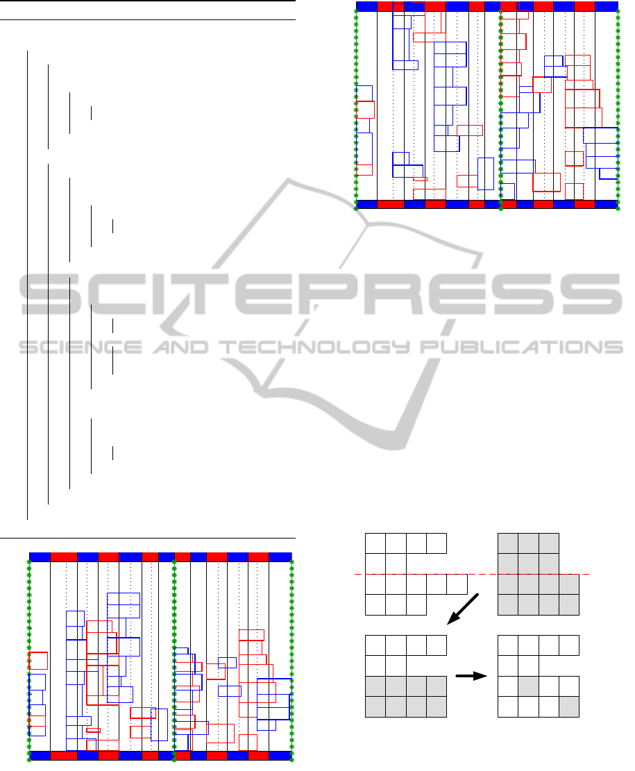
Individual Representation. An individual represents
one possible solution for the BAP-C and it is de-
scribed as a matrix with the lines indicating the berths
and the columns presenting the sequence of ships to
be handling at each berth. Figure 4 illustrates an in-
dividual (solution) for a hypothetical problem with 4
berths and 14 ships.
4
2
7
11
10
9
1
14
6
3
5
8 12
13Berth 1
Berth 4
Berth 3
Berth 2
Figure 4: Individual representation.
Initial Population. A random individual can be con-
structed through a simple and balanced heuristic. Ini-
tially, the ships are organized by incoming order on
port (a
i
) and distributed to the berths in a random
way. In this process, the selected berth must always
be able to assist the selected ship. This procedure en-
sures that each ship will be assigned to a berth that
must be able to attend it, i.e., the berth length is suf-
ficient to receive the ship and the berth’s equipments
are suitable to operate the type of cargo into the ship.
So, this procedure is repeated for #pop times forming
an initial population. This procedure does not guaran-
tee that the berthing time (T
i
) and position (P
i
) for the
ship i (i = 1, . . . , n) present no overlappingon time and
space dimensions. This strategy is based on the dis-
tribution heuristic presented by Mauri et al. (2008a,b)
and the FCFS-G heuristic presented by Cordeau et al.
(2005).
Computing Berthing Times and Positions. After
generating a random individual (solution), we must
define the berthing time and position for all of ships.
We present a two-phase heuristic to determine these
values.
• Phase 1: Berthing time and position for all of
ships assigned to a specific berth are set to initial
values according to Algorithm 2. At this moment,
the berthing times are set to equal the arrival times
of the ships, if the berth is available. The berthing
positions are set to equal the start position of the
berth. This phase is applied to give initial values
for P
i
and T
i
, that are updated in phase 2. This pro-
cedure is based on the ones presented by Mauri
et al. (2008a,b), Pacheco et al. (2010) and Ribeiro
et al. (2011) adding the position defining.
Algorithm 2: Two-phase heuristic - phase 1.
1 Input: berth k
2 for each ship i assigned to k do
3 T
i
←
(
max
a
i
,s
k
i = 1
max
a
i
,T
i−1
+t
k
i−1
i > 1
4 P
i
← P
s
k
5 end
• Phase 2: The spatial distribution for the ships to
the berths are updated and improved. This proce-
dure updates the berthing times and positions con-
sidering a simple idea: if some overlap is detected
for each ship, its berthing time is delayed until
eliminate all of them. If a berth has no neighbor
at the left side, all of ships assigned to it have the
berthing position set to equal the start position of
the berth, i.e., all of ships (rectangles) are aligned
at left. If a berth has no neighbor at the right side,
all of ships assigned to it have the berthing po-
sition set to equal the final position of the berth
minus the ship length, i.e., all of ships are aligned
at right. Finally, if a berth has neighbors on both
sides, we try to fit the ships among the ones as-
signed to the two neighbor berths. This procedure
is described in Algorithm 3.
Figures 5 and 6 illustrate a randomly generated in-
dividual after running only phase 1 and after phases 1
and 2 of our two-phase heuristic.
In the first case (Figure 5), only the phase 1 of our
heuristic was performed, and we can note that over-
lapping were not treated. In the second case (Figure
6), both phases were computed and no overlapping is
presented. However, we can observe that some ships
violate the deadlines for some berths (see berths 2, 3,
4, 8 and 9), and these violations must be eliminated by
our MA through a penalized objective function (see
expression 1).
A MEMETIC ALGORITHM FOR A CONTINUOUS CASE OF THE BERTH ALLOCATION PROBLEM
109
Algorithm 3: Two-phase heuristic - phase 2.
1 Input: berth k
2 for each ship i assigned to k do
3 if L
k
= 0 then
4 P
i
← P
s
k
5 for each ship j assigned to k+ 1 do
6 if i overlaps j then
7 T
i
← max(T
i
,T
j
+t
k+1
j
)
8 end
9 end
10 else
11 if R
k
= 0 then
12 P
i
← P
f
k
− z
i
13 for each ship j assigned to k− 1 do
14 if i overlaps j then
15 T
i
← max(T
i
,T
j
+t
k−1
j
)
16 end
17 end
18 else
19 P
i
← P
s
k
20 while ∃ j assigned to k− 1 overlapping i do
21 if (P
j
+ z
j
≥ P
s
k
) and (P
j
+ z
j
+ z
i
≤ P
f
k
) then
22 P
i
← P
j
+ z
j
23 else
24 T
i
← max(T
i
,T
j
+t
k−1
j
)
25 P
i
← P
f
k
− z
i
26 end
27 end
28 while ∃ j assigned to k+ 1 overlapping i do
29 T
i
← max(T
i
,T
j
+t
k+1
j
)
30 while ∃ l assigned to k− 1 overlapping i do
31 T
i
← max(T
i
,T
l
+t
k−1
l
)
32 end
33 end
34 end
35 end
36 end
0
50
100
150
200
250
300
SPACE
TIME
B1
B1
B2
B2
B3
B3
B4
B4
B5
B5
B6
B6
B7
B7
B8
B8
B9
B9
B10
B10
B11
B11
B12
B12
B13
B13
Figure 5: Random solution after phase 1.
Individual Evaluation. We may notice that our two-
phase heuristic guarantees that no overlapping will
occur and no ship will exceed the spatial limit of the
berths. However, our solutions can still present viola-
0
50
100
150
200
250
300
SPACE
TIME
B1
B1
B2
B2
B3
B3
B4
B4
B5
B5
B6
B6
B7
B7
B8
B8
B9
B9
B10
B10
B11
B11
B12
B12
B13
B13
Figure 6: Random solution after phases 1 and 2.
tions on the limit time to complete the service of the
ships (b
i
,∀i = 1,... , n) and on the end of availability
time of the berths (e
k
,∀k = 1,...,m). So, we define a
function to compute the cost of an individual consid-
ering a weight λ to penalty theses violations (see ex-
pression 1). This function is composed by three terms
representing the service times for the ships (sum of
the times when the ships stayed in port) and the sum
of violating deadlines for the ships and berths respec-
tively. The fitness measure used to evaluate the indi-
viduals was 1/ f(I).
f(I) =
∑
k∈M
∑
i∈N
T
i
+ t
k
i
− a
i
+
λ
∑
k∈M
∑
i∈N
max
0,T
i
+ t
k
i
− b
i
+
λ
∑
k∈M
∑
i∈N
max
0,T
i
+ t
k
i
− e
k
(1)
4
2
7
11
10
9
1
14
6
3
5
8 12
13 2
10
5
14
11
4
6
7
9
3
12
8
13
1
4
2
5
14
10
9
7
6
3
12
8
13 4
2
5
14
10
9
11
7
6
3
12
8
1
13
p
1
p
2
off
off
Figure 7: Crossover.
Crossover. A one-point based crossover was im-
plemented. Given two parents p
1
and p
2
, a number
of berths x (0 < x < m) is randomly selected and
then the first x berths from p
1
are inserted into the
offspring of f. Then, the last m − x berths from p
2
are inserted into of f removing the duplicated ships,
and the ships that have not been assigned to any berth
ECTA 2011 - International Conference on Evolutionary Computation Theory and Applications
110

are randomly allocated at the last m− x berths in of f.
The ships assigned to each of the last m − x berths
are organized by incoming order on port (a
i
) and the
two-phase heuristic is applied only to these berths in
of f. Finally, function 1 is used to compute the cost
(f(of f)) and fitness for of f (1/ f(o f f )). Figure 7
illustrates our crossover.
Mutation. Three different procedures explored in
previous works (see Mauri et al. (2008a), Pacheco
et al. (2010) and Ribeiro et al. (2011)) were used
to compose a neighborhood structure: Re-order
ships, Re-allocate ship and Swap ships. We will
denote them as ω
1
, ω
2
and ω
3
respectively. ω
1
is
obtained by randomly choosing two ships of the
same berth, and swapping them; ω
2
is obtained by
inserting a ship i chosen at random from some berth
into another berth in a position chosen at random;
and ω
3
is obtained by swapping two ships from two
different berths, all chosen at random. So, a mutation
is defined by applying one of these procedures
(randomly selected) over an individual followed
by performing the two-phase heuristic on the modi-
fied berths. Finally, the individual’s fitness is updated.
Local Search. A traditional Simulated Annealing
(SA) presented in previous works (see Ribeiro et al.
(2011)) was used as the local search mechanism for
our Memetic Algorithm (MA). The neighborhood
structure for our SA were composed by selecting (at
random) one of the three procedures adopted in the
Mutation. We must emphasize that low values for the
SA parameters were used into our MA to make only a
fast local search. These parameters values were: α =
0.95, T
start
= 10, T
frozen
= 0.01 and SA
max
= #ls (de-
fined in the next section).
5 COMPUTATIONAL RESULTS
This section presents a comparative evaluation of our
Memetic Algorithm (MA) and Simulated Annealing
(SA) applied in a stand alone way. Both heuristics
were applied 10 times to each instance, and to be fair,
we imposed a time limit as unique stopping criterion
for them: 120 seconds for each instance, i.e., the same
time used by Tabu Search (TS) proposed by Cordeau
et al. (2005).
The SA and MA heuristics have stopping condi-
tions based on the temperature and on the number of
generations, respectively. If they reach their stopping
conditions before the time limit, we restart the heuris-
tic from the best solution identified during the search.
This process is repeated until the heuristic reaches the
time limit.
The SA and MA heuristics were coded in C++
and ran on a PC with Intel Core i3 processor of 2.66
GHz with 4 GB of RAM Memory under Windows
7 operating system. Cordeau et al. (2005) had use a
Sun workstation (900 MHz) to run their TS. Our algo-
rithms were tested on a BAP instances set randomly
generated by Cordeau et al. (2005). This set is com-
posed by 30 different instances with 60 ships and 13
berths, and it was provided to us by the authors in a
previous situation.
The parameters of SA and MA were chosen em-
pirically after running them over three randomly se-
lected instances. We ran SA and MA five times for
each parameter setting, and the setting yielding the
best average results was chosen. So, the final values
for the SA parameters were: T
start
= 15000, T
frozen
=
0.01, α = 0.975, SA
max
= 1000. The parameters for
our MA were: #pop = 30, #eli = 10, #cro = 25, #mut
= 5 and #ls = 7. The parameters used by SA (as a
local search) inside the MA were defined in Section
4.
A special attention was given to the weight λ, be-
cause we note that a large value for this weight often
traps the search in a locally suboptimal solution. So,
the weight value was set to 10 (λ = 10).
Table 1: Results from our SA and MA heuristics.
SA MA
Instance f(I
∗
) Time (s) f(I
∗
) Time (s)
bst avge bks bst bst avge bks bst
i01 1639 1661.60 21.45 58.45 1613 1666.50 37.49 85.41
i02
1326 1341.20 28.17 41.47 1326 1347.80 51.91 75.85
i03
1242 1254.90 28.12 58.51 1234 1261.90 20.58 79.99
i04
1392 1416.40 31.79 65.63 1392 1421.00 36.36 84.54
i05
1285 1300.80 16.53 91.54 1285 1302.00 8.55 90.02
i06
1461 1492.00 17.28 67.69 1461 1492.10 5.84 85.67
i07
1333 1347.10 19.48 64.68 1333 1352.00 12.38 92.50
i08
1425 1470.30 34.69 80.23 1425 1466.40 12.88 91.94
i09
1651 1693.80 55.22 59.20 1651 1698.20 40.06 89.57
i10
1371 1380.40 40.67 61.45 1371 1393.00 38.93 72.64
i11
1574 1606.50 20.82 59.57 1557 1602.10 5.70 72.93
i12
1541 1568.60 22.21 56.87 1537 1565.80 7.64 88.01
i13
1457 1468.60 18.39 47.73 1449 1482.50 23.66 83.02
i14
1284 1289.80 16.98 58.90 1287 1306.90 6.57 80.19
i15
1362 1376.50 19.10 65.92 1362 1394.20 14.44 75.85
i16
1508 1539.00 14.49 70.45 1508 1581.10 4.28 87.78
i17
1310 1321.40 52.24 54.70 1318 1335.30 68.71 83.41
i18
1529 1549.10 25.59 59.68 1519 1552.10 21.68 89.47
i19
1572 1614.60 33.32 62.10 1573 1628.60 26.00 84.78
i20
1438 1456.40 52.98 50.21 1428 1469.30 67.47 91.01
i21
1478 1494.80 16.03 86.28 1481 1510.40 7.64 80.47
i22
1484 1519.00 22.22 78.94 1484 1521.00 12.57 86.19
i23
1425 1456.00 23.58 54.52 1425 1456.10 3.56 84.86
i24
1365 1375.30 15.99 73.48 1359 1383.40 14.40 87.65
i25
1546 1578.20 45.12 53.87 1546 1604.50 38.04 79.12
i26
1475 1507.40 30.07 62.51 1475 1520.10 22.25 80.51
i27
1356 1371.50 15.39 88.81 1356 1382.30 6.59 70.23
i28
1504 1525.20 44.35 69.11 1486 1553.90 53.80 81.15
i29
1340 1351.20 16.03 55.84 1338 1360.80 6.76 74.49
i30
1512 1547.30 15.17 82.53 1512 1555.60 7.43 84.63
Avge 1439.50 1462.50 27.11 64.70 1436.37 1472.23 22.81 83.13
Table 1 presents a detailed comparison between
our SA and MA performance. Five different columns
are used for all results: the instance name, the best so-
A MEMETIC ALGORITHM FOR A CONTINUOUS CASE OF THE BERTH ALLOCATION PROBLEM
111
lution found (f(I
∗
) → bst), the averagesolution found
(avge), the computational time (bks) to reach the best-
known so far (TS by Cordeau et al. (2005)) and the
computational time to found the best solution for each
algorithm (Times(s) → bst).
In Table 1, we can note that MA found ten best
solutions and four worse than SA. The others sixteen
solutions were equal. Despite the differences, we no-
tice that MA is slightly better, but in general, the so-
lutions of SA and MA are very close. This fact can
indicate that our solutions are probably next to the
optimal ones. We confirmed this situation in Tabel
3. The average values (last line) are also close, and
we emphasize that our heuristics find the same solu-
tions of TS proposed by Cordeau et al. (2005) using
less than 30 seconds.
Table 2: Comparison with the TS of Cordeau et al. (2005).
TS SA MA
Instance
bst dev (%) bst dev (%) bst dev (%)
i01 1706 5.77 1639 1.61 1613 0
i02 1355 2.19 1326 0 1326 0
i03
1286 4.21 1242 0.65 1234 0
i04 1440 3.45 1392 0 1392 0
i05
1352 5.21 1285 0 1285 0
i06
1565 7.12 1461 0 1461 0
i07 1389 4.20 1333 0 1333 0
i08
1519 6.60 1425 0 1425 0
i09 1713 3.76 1651 0 1651 0
i10
1411 2.92 1371 0 1371 0
i11 1696 8.93 1574 1.09 1557 0
i12
1629 5.99 1541 0.26 1537 0
i13 1519 4.83 1457 0.55 1449 0
i14
1369 6.62 1284 0 1287 0.23
i15
1455 6.83 1362 0 1362 0
i16 1715 13.73 1508 0 1508 0
i17
1322 0.92 1310 0 1318 0.61
i18 1594 4.94 1529 0.66 1519 0
i19
1673 6.42 1572 0 1573 0.06
i20 1450 1.54 1438 0.70 1428 0
i21
1565 5.89 1478 0 1481 0.20
i22 1618 9.03 1484 0 1484 0
i23
1539 8.00 1425 0 1425 0
i24
1425 4.86 1365 0.44 1359 0
i25 1590 2.85 1546 0 1546 0
i26
1567 6.24 1475 0 1475 0
i27 1458 7.52 1356 0 1356 0
i28
1550 4.31 1504 1.21 1486 0
i29 1415 5.75 1340 0.15 1338 0
i30
1621 7.21 1512 0 1512 0
Avge 1516.87 5.59 1439.50 0.24 1436.37 0.04
Table 2 presents a comparison among our algo-
rithms and the Tabu Search by Cordeau et al. (2005).
The columns present the best solutions found (bst)
by each heuristic and their deviations (dev(%)). The
deviations are calculated as dev(%) = 100 × (bst −
bst
∗
)/bst
∗
, where bst
∗
is the best-known solution
value obtained by any of the three heuristics for a
given instance. We can observe that both SA and MA
found better solutions than TS for all of instances, and
MA presents better solutions than SA.
Table 3 shows the gaps over the lower bounds
(BAP-D) presented by Buhrkal et al. (2011). The
column OPT BAP-D reports the optimal solutions
(proven by Buhrkal et al. (2011)) for the discrete case
of BAP. As mentioned before, according to Cordeau
et al. (2005) and Imai et al. (2005), solutions for
the BAP-D are lower bounds for the BAP-C. The
gaps shown in the last columns are calculated as
Gaps(%) = 100× (X −Y)/Y, where X is the best so-
lution found by each of three heuristics for the BAP-C
and Y is the value for the lower bound (OPT BAP-D).
Table 3: Comparison with the optimal solutions for BAP-D.
OPT BAP-C Gaps (%)
Instance
BAP-D TS SA MA BT SA MA
i01 1409 1706 1639 1613 21.08 16.32 14.48
i02
1261 1355 1326 1326 7.45 5.15 5.15
i03
1129 1286 1242 1234 13.91 10.01 9.30
i04 1302 1440 1392 1392 10.60 6.91 6.91
i05
1207 1352 1285 1285 12.01 6.46 6.46
i06 1261 1565 1461 1461 24.11 15.86 15.86
i07
1279 1389 1333 1333 8.60 4.22 4.22
i08 1299 1519 1425 1425 16.94 9.70 9.70
i09
1444 1713 1651 1651 18.63 14.34 14.34
i10 1213 1411 1371 1371 16.32 13.03 13.03
i11
1368 1696 1574 1557 23.98 15.06 13.82
i12 1325 1629 1541 1537 22.94 16.30 16.00
i13
1360 1519 1457 1449 11.69 7.13 6.54
i14
1233 1369 1284 1287 11.03 4.14 4.38
i15 1295 1455 1362 1362 12.36 5.17 5.17
i16
1364 1715 1508 1508 25.73 10.56 10.56
i17 1283 1322 1310 1318 3.04 2.10 2.73
i18
1345 1594 1529 1519 18.51 13.68 12.94
i19 1367 1673 1572 1573 22.38 15.00 15.07
i20
1328 1450 1438 1428 9.19 8.28 7.53
i21 1341 1565 1478 1481 16.70 10.22 10.44
i22
1326 1618 1484 1484 22.02 11.92 11.92
i23 1266 1539 1425 1425 21.56 12.56 12.56
i24
1260 1425 1365 1359 13.10 8.33 7.86
i25
1376 1590 1546 1546 15.55 12.35 12.35
i26 1318 1567 1475 1475 18.89 11.91 11.91
i27
1261 1458 1356 1356 15.62 7.53 7.53
i28 1359 1550 1504 1486 14.05 10.67 9.35
i29
1280 1415 1340 1338 10.55 4.69 4.53
i30 1344 1621 1512 1512 20.61 12.50 12.50
Avge 1306.77 1516.87 1439.50 1436.36 16.0 10.1 9.8
Looking at Table 3, it is interesting to highlight
the gaps over the optimal solutions for the BAP-D.
We can verify that our MA solutions are relatively
close to the optimal, because the average gap was of
9.8%. We may also note a significant reduction over
the solutions provided by the Tabu Search proposed
by Cordeau et al. (2005).
6 CONCLUSIONS
In this paper we have developed a Memetic Algorithm
(MA) to solve a continuous case of the Berth Alloca-
tion Problem (BAP).
MA was employed by using a Simulated Anneal-
ing (SA) as the local search mechanism and a two-
phase heuristic to compute the berthing time and po-
ECTA 2011 - International Conference on Evolutionary Computation Theory and Applications
112

sition for all of ships. SA was also applied in a stand
alone way.
On test instances, both SA and MA yield good re-
sults and outperform the rather good Tabu Search of
Cordeau et al. (2005). Our results show a relative su-
periority of the MA, but SA also found good solu-
tions.
The integrated use of MA, SA and the two-phase
heuristic results in a powerful approach to solve the
continuous case of the BAP, providing good solutions
in low computational times.
MA showed to be extremely efficient, presenting
small gaps over the best-known lower bounds and
suggesting that our solutions are probably close to op-
timal.
So, considering that the continuous case of the
BAP represents real situations in a more appropriate
way, and considering that BAP has a significant im-
pact on the efficiency of the marine terminals, a mini-
mal reduction on the service times may reflects a gain
and/or economy of millions of dollars.
ACKNOWLEDGEMENTS
The authors acknowledge Esp´ırito Santo Research
Foundation - FAPES (process 45391998/09) and
National Council for Scientific and Technological
Development - CNPq (processes 300747/2010-1,
300692/2009-9 and 470813/2010-5) for their finan-
cial support.
REFERENCES
Barros, V. H., Costa, T. S., Oliveira, A. C. M., and Lorena,
L. A. N. (2011). Model and heuristic for berth allocation
in tidal bulk ports with stock level constraints. Comput-
ers & Industrial Engineering, 60:606–613.
Buhrkal, K., Zuglian, S., Ropke, S., Larsen, J., and Lusby,
R. (2011). Models for the discrete berth allocation
problem: a computational comparison. Transportation
Research Part E: Logistics and Transportation Review,
47:461–473.
Cordeau, J. F., Laporte, G., Legato, P., and Moccia, L.
(2005). Models and tabu search heuristics for the berth
allocation problem. Transportation Science, 39:526–
538.
Dragovic, B., Park, N. K., and Radmilovic, Z. (2005). Sim-
ulation modelling of ship-berth link with priority service.
Maritime Economics & Logistics, 7:316–335.
Giallombardo, G., Moccia, L., Salani, M., and Vacca, I.
(2010). Modeling and solving the tactical berth alloca-
tion problem. Transportation Research Part B, 44:232–
245.
Hansen, P., Oguz, C., and Mladenovic, N. (2008). Variable
neighborhood search for minimum cost berth allocation.
European Journal of Operational Research, 191:636–
649.
Imai, A., Nishimura, E., and Papadimitriou, S. (2001).
The dynamic berth allocation problem for a container
port. Transportation Research Part B: Methodological,
35:401–417.
Imai, A., Nishimura, E., and Papadimitriou, S. (2003).
Berth allocation with service priority. Transportation Re-
search Part B: Methodological, 37:437–457.
Imai, A., Sun, X., Nishimura, E., and Papadimitriou, S.
(2005). Berth allocation in a container port: using a
continuous location space approach. Transportation Re-
search Part B, 39:199–221.
Mauri, G. R., Oliveira, A. C. M., and Lorena, L. A. N.
(2008a). Heur´ıstica baseada no simulated annealing apli-
cada ao problema de alocac¸˜ao de berc¸os. GEPROS -
Gest˜ao da Produc¸˜ao, Operac¸˜oes e Sistemas, 1:113–127.
Mauri, G. R., Oliveira, A. C. M., and Lorena, L. A. N.
(2008b). A hybrid column generation approach for the
berth allocation problem. Lecture Notes in Computer Sci-
ence, 4972:110–122.
Moscato, P. (1999). Memetic algorithms: a short introduc-
tion. In Corne, D., Dorigo, M., Glover, F., Dasgupta, D.,
Moscato, P., Poli, R., and Price, K. V., editors, New ideas
in optimization. 219–234.
Moscato, P. and Norman, M. (1992). A memetic approach
for the travelling salesman problem: implementation of
a computational ecology for combinatorial optimization
on message-passing systems. In Proceedings of the Inter-
national Conference on Parallel Computing and Trans-
portation Applications. 177–186.
Nishimura, E., Imai, A., and Papadimitriou, S. (2001).
Berth allocation planning in the public berth system by
genetic algorithms. European Journal of Operational
Research, 131:282–292.
Pacheco, A. V. F., Ribeiro, G. M., and Mauri, G. R. (2010).
A grasp withpath-relinking for the workover rig schedul-
ing problem. International Journal of Natural Comput-
ing Research, 1:1–14.
Ribeiro, G. M., Mauri, G. R., and Lorena, L. A. N. (2011).
A simple and robust simulated annealing algorithm for
scheduling workover rigs on onshore oil fields. Comput-
ers & Industrial Engineering, 60:519–526.
Steenken, D., Voss, S., and Stahlbock, R. (2004). Container
terminal operation and operations research: a classifica-
tion and literature review. OR Spectrum, 26:3–49.
UNCTAD (2009). Review of maritime transport. United
Nations conference on trade and development.
Vis, I. F. A. and Koster, R. D. (2003). Transshipment of
containers at a container terminal: an overview. Euro-
pean Journal of Operational Research, 147:1–16.
A MEMETIC ALGORITHM FOR A CONTINUOUS CASE OF THE BERTH ALLOCATION PROBLEM
113
