
AN INNOVATIVE PROTOCOL FOR COMPARING PROTEIN
BINDING SITES VIA ATOMIC GRID MAPS
M. Bicego
1,2
, A. D. Favia
3
, P. Bisignano
3
, A. Cavalli
3
and V. Murino
1,2
1
PLUS Lab, Istituto Italiano di Tecnologia, I-16163 Genoa, Italy
2
Dipartimento di Informatica, University of Verona, I-37134 Verona, Italy
3
Department of Drug Discovery and Development (D3), Istituto Italiano di Tecnologia, I-16163 Genoa, Italy
Keywords:
Protein similarity, 3D points alignment, Iterative closest point, Drug design, Multitarget.
Abstract:
This paper deals with a novel computational approach that aims to measure the similarities of protein binding
sites through comparison of atomic grid maps. The assessment of structural similarity between proteins is a
longstanding goal in biology and in structure-based drug design. Instead of focusing on standard structural
alignment techniques, mostly based on superposition of common structural elements, the proposed approach
starts from a physicochemical description of the proteins’ binding site. We call these atomic grid maps. These
maps are preprocessed to reduce the dimensionality of the data while retaining the relevant information. Then,
we devise an alignment-based similarity measure, based on a rigid registration algorithm (the Iterative Closest
Point –ICP). The proposed approach, tested on a real dataset involving 22 proteins, has shown encouraging
results in comparison with standard procedures.
1 INTRODUCTION
In this paper, we address a fundamental issue in
structural biology and in structure-based drug design,
namely the characterization, for comparative pur-
poses, of a set of macromolecular entities such as pro-
teins (Kahraman and Thornton, 2008). Since struc-
ture is more conserved than sequence, the most com-
mon approaches rely on the superposition of common
structural elements. Such methods allow researchers
to compare, with an increasing degree of difficulty,
a) different conformations of the same protein, b)
homologous proteins and, c) evolutionarily-unrelated
proteins.
Traditionally, structural alignment techniques rely
on the punctual superposition of correspondent atoms,
usually the protein backbones or C-α, in different
entries (Shindyalov and Bourne, 1998; Holm and
Sander, 1993). A more sophisticated class of pro-
tocols considers elements of the protein secondary
structures (Jung and Lee, 2000; Chen and Crippen,
2005; Kawabata, 2003). However, these reductionist
approaches, based on geometric hashing, do not take
into account the physicochemical complexity of the
systems. This is because they completely ignore the
fields produced by the macromolecule (e.g. the ones
experienced by interacting molecules) (Favia, 2011).
Furthermore, these methods cannot be safely applied
to evolutionarily-distant proteins, due to the lack of
sound correspondences between atoms.
To overcome these limits, we herein introduce a
new protocol, based on van der Waals potential en-
ergies (IUPAC, 1997) calculated at regularly spaced
points within a predefined volume. The definition of
the volume is case-specific and is usually defined ac-
cording to the binding site definition. This method
allows one a) to compare binding sites and, in a more
advanced application, b) to guide a more physico-
chemically sound structure alignment. Van der Waals
interactions between nonbonded atoms can be ex-
pressed as a function of their internuclear separation
through the Lennard-Jones equations. At each of the
regularly spaced points, a virtual atom type is placed
and its potential is evaluated. This atom type can be
thought of as a chemical probe that experiences the
protein fields. The energy at each grid point is deter-
mined by the set of parameters supplied for that par-
ticular probe, and is estimated as the summation over
all atoms of the macromolecule, within a non-bonded
cutoff radius, of all pairwise interactions. Different
probes experience different fields, according to their
assigned chemical features. Taken together, a mini-
mal set of selected probes, namely carbon, oxygen,
and hydrogen atoms, can give a useful description of
the studied volume based on shape (C probe), H-bond
donor, and acceptor propensity (H and O probes, re-
spectively) (see Fig. 1). Once this physicochemi-
cal description of the volume is achieved, it can be
413
Bicego M., D. Favia A., Bisignano P., Cavalli A. and Murino V..
AN INNOVATIVE PROTOCOL FOR COMPARING PROTEIN BINDING SITES VIA ATOMIC GRID MAPS.
DOI: 10.5220/0003637404050414
In Proceedings of the International Conference on Knowledge Discovery and Information Retrieval (KDIR-2011), pages 405-414
ISBN: 978-989-8425-79-9
Copyright
c
2011 SCITEPRESS (Science and Technology Publications, Lda.)
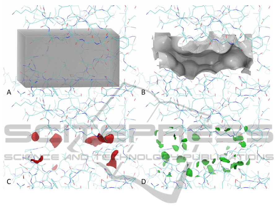
Figure 1: Grid point generation. An enclosing box is defined within a protein active site (A). The grid maps can then be
conveniently visualize as isocontour maps. The carbon, oxygen and hydrogen maps are shown in (B), (C) and (D) at 0, -1 and
-0.6 kcal/mol isocontour level, respectively. The protein structure is shown in the background of the 4 panels.
used to compare a) different conformations of the
same protein and b) different proteins altogether. The
presented protocol is similar in spirit to the recently
developed protocol for ligand-binding site superposi-
tion and comparison based on Atomic Property Fields
(Totrov, 2011).
This paper introduces a computational approach
able to compare two or more proteins starting from
the above-mentioned physicochemical description of
their binding site. We call these descriptions atomic
grid maps. In particular, the idea is to exploit tech-
niques from the Computer Vision and Pattern Recog-
nition fields to devise similarity between maps in or-
der to understand and highlight relations between dif-
ferent proteins.
The computation of the similarity is carried out
in two steps: first, a chemically plausible prepro-
cessing transforms the real-valued potential maps into
discrete-valued maps (which we call ”meta-maps”);
then, the meta-maps are compared using a rigid align-
ment algorithm (the Iterative Closest Point – ICP
((Besl and McKay, 1992; Chen and Medioni, 1992)),
setting the distance between the pair of proteins as the
alignment error. This alignment may be performed
either by using a single value of the meta-map or by
combining together all the values. A similarity clearly
expresses the relation between two proteins: a more
general view may be obtained by taking a set of pro-
teins, computing all the pairwise distances, and visu-
alizing all the relations through a hierarchical cluster-
ing approach (Jain and Dubes, 1988).
The proposed approach has been applied to a real
dataset composed of diverse X-ray structures of GSK-
3β, a protein involved in Alzheimer’s disease (Her-
nandez et al., 2009), as extracted from the Worldwide
Protein Data Bank (wwPDB) (Berman et al., 2003).
The similarity measures obtained with the proposed
approach have been compared with those obtained
through a time-consuming computational procedure
based on the comparison of structure-assisted virtual
screening ranked distributions (Bottegoni et al., 2011)
(which can be considered as the ”true” distances). We
will show in our experiments that the proposed com-
putational method can approximate these true dis-
tances in an encouraging way.
We note that this could be an invaluable drug
KDIR 2011 - International Conference on Knowledge Discovery and Information Retrieval
414

design tool. This is because representative confor-
mations of a studied protein could be used to run
time-demanding molecular simulations (e.g. dock-
ing), rather than using the whole ensemble of avail-
able structures. More broadly, when applied to un-
related proteins, the methodology could conveniently
highlight common hotspots that could be exploited
to design multitarget drugs (i.e. molecules capable
of binding different proteins). These are particu-
larly useful in treating complex diseases (Morphy and
Rankovic, 2006).
The remainder of the paper is organized as fol-
lows: Section 2 describes how potentials maps are
extracted. In Section 3, we present the proposed ap-
proach. Section 4 describes an experimental evalua-
tion that validates the methodology. Finally, in Sec-
tion 5, conclusions are drawn and future perspectives
are envisaged.
2 POTENTIAL MAPS
The active sites of the selected structures of GSK-3β
were first superimposed using the McLachlan algo-
rithm (McLachlan, 1982) as implemented in the pro-
gram ProFit
1
. Then, van der Waals forces were com-
puted, using the AutoGrid software as distributed with
AutoDock4.2 (Morris et al., 2009). AutoGrid solves
the Lennard-Jones equations at regularly spaced grid
points (0.375
˚
A) enclosed in a box centered on the
center of mass of the atoms belonging to the active
site, spanning 14.25, 11.25 and 21
˚
A along the three
axes. To give an accurate description of the site, three
diverse atom probes were placed at each node of the
grid to sense the protein environment, namely the car-
bon, hydrogen and oxygen probes. In particular, the
carbon probe accounts for the shape and hydropho-
bic features of the binding site, while the hydrogen
and the oxygen probes account for the hydrogen bond
propensity. Pairwise atomic interactions are approxi-
mated through the following equation:
V (r) =
C
n
r
n
−
C
m
r
m
= C
n
r
−n
− C
m
r
−m
(1)
Here, m and n are integers, C
n
and C
m
are constants
whose values vary according to the type of atoms and
probes involved and r is the distance between them.
At distances shorter than the equilibrium distance (in
correspondence to the minimum of the function), the
potential energy function increases rapidly (i.e. the
probe clashes with the protein), while at long dis-
tances the function tends to zero (i.e. the probe does
not feel the presence of the protein).
1
A.C.R. Martin http://www.bioinf.org.uk/software/profit/
3 THE PROPOSED APPROACH
The goal of the proposed approach is to characterize
a set of proteins, each one described by a set of poten-
tials maps. The idea is to highlight the relations be-
tween the different proteins of the chosen set by de-
vising a similarity measure, which could potentially
be used in a clustering scenario to highlight all the
possible relations. Some different distances are de-
fined and described in Sect. 3.2. These are all based
on a chemically sound preprocessing algorithm used
to simplify the potential maps, as described in the next
Section.
3.1 Preprocessing of Data: The
Meta-maps
AutoGrid produces real-valued potential maps. As
such, they are difficult to interpret. Hence, we parsed
the three Auto-Grid readouts to yield a single map that
retains all the relevant information. A few considera-
tions must be made here:
• the oxygen and hydrogen probes are mutually ex-
clusive;
• both are considered to be more relevant, from a
chemical perspective, than the carbon probe;
• we were only interested in negative values (i.e.
when probes and protein do not clash)
• after a heuristically defined cutoff, small differ-
ences in potential energies are negligible.
Bearing this in mind, every position of the potential
maps may be described with one of four different val-
ues:
• value ’1’: if the oxygen probe, in this posi-
tion, recorded a potential energy lower than -1
kcal/mol;
• value ’-1’: if the hydrogen probe, in this position,
recorded a value lower than -0.6 kcal/mol;
• value ’0’: if the carbon probe, in this position,
recorded any negative value of the potential en-
ergy function;
• no value if none of the above criteria were fulfilled
in this position;
In doing so, a net compression of the data is possi-
ble, yet the relevant information is retained and con-
veniently encoded into a single, ternary grid map.
3.2 Devising the Similarity
Once the meta-maps have been obtained, the next step
is to define the similarity measure. One reasonable
AN INNOVATIVE PROTOCOL FOR COMPARING PROTEIN BINDING SITES VIA ATOMIC GRID MAPS
415

strategy is to link the similarity to the alignment of
the meta-maps, in order to measure, in some sense,
how dissimilar two maps remain after maximizing the
overlap between them (it may also be seen as the op-
posite of the overlap ratio between two maps).
In particular, we investigated two different ap-
proaches:
1. Alignment based on a Single Value. Here, we
selected only those meta-maps points with a spe-
cific value (-1, 0 or 1). In this way, the alignment
was transformed into a simpler problem of regis-
tration of point clouds – where the term ”registra-
tion” describes the geometric alignment of a pair
of 3D data-point sets. This is a well-known prob-
lem in computer vision (Trucco and Verri, 1998),
and many techniques to solve it have been pro-
posed in the past. One of the most famous is the
Iterative Closest Point (ICP – (Besl and McKay,
1992; Chen and Medioni, 1992)), briefly summa-
rized later in this section;
2. Alignment based on all Values. The distance
was computed by simultaneously using all the val-
ues of the metamaps.
Before entering into the details, we will review
the Iterative Closest Point (ICP) algorithm (Besl and
McKay, 1992; Chen and Medioni, 1992).
3.2.1 Iterative Closest Point Algorithm
Let us suppose that we have two sets of 3D points,
V
i
and V
j
. The registration consists of finding a 3D
transformation which, when applied to V
j
, minimizes
the distance between the two point sets. In general,
point correspondences are unknown. For each point
y
i
from the set V
j
, there exists at least one point on
the surface of V
i
that is closer to y
i
than all the other
points in V
i
. This is the closest point, x
i
. The basic
idea behind the ICP algorithm is that, under certain
conditions, closest points are a reasonable approxi-
mation to the true point correspondences. The ICP
algorithm can be summarized as follows:
1. For each point in V
j
, compute the closest point in
V
i
;
2. With the correspondence from step 1, compute the
incremental transformation (R
i, j
, t
i, j
);
3. Apply the incremental transformation from step 2
to the set V
j
;
4. If the change in total mean square error is less than
a threshold, terminate. Otherwise, go to step 1.
Besl and McKay (Besl and McKay, 1992) proved
that this algorithm is guaranteed to converge mono-
tonically to a local minimum of the mean square error.
Thus, a good initialization is required. To overcome
this problem, we manually pre-aligned the proteins
in our experiments. For step 2, efficient, noniterative
solutions to this problem (known as the point set reg-
istration problem) were compared in (Lorusso et al.,
1997). The solution based on singular value decom-
position was found to be the best in terms of accuracy
and stability.
After the convergence of the algorithm, the total
mean square error represents the registration error be-
tween the two sets of points.
After the convergence of the algorithm, the total
mean square error represents the registration error be-
tween the two sets of points.
3.2.2 Single Value Analysis
Given two proteins to be compared, the distance is
computed via the following steps:
1. for every protein, the three potential maps are
preprocessed to produce the corresponding meta-
map;
2. from the meta-map, only points with a specific
value are extracted (for example, all points with
’0’ value). This results in a cloud of 3D points;
3. the two 3D point clouds (relative to the two pro-
teins) are registered through the ICP algorithm.
The registration error represents the final distance.
3.2.3 Multiple Values Analysis
The previous approach is of course limited by the fact
that the meta-maps are decomposed in three different
non-overlapping sets, which are used alone – in this
sense using only partial information. It seems reason-
able, therefore, to try to develop a method that can
integrate and use all the information present in the
meta-maps. From a very general Pattern Recognition
point of view, this problem may be contextualized
in the Multiclassifier theory (also called Multimodal
or Fusion theory, depending on the context). These
theories aim to integrate the potentially complemen-
tary information provided by different methodolo-
gies/representations in a particular problem, by ex-
ploiting the different peculiarities of the fused tech-
niques. This theory, first introduced in the classifi-
cation context (Ho et al., 1994; Kittler et al., 1998;
Melnik et al., 2004) and, more recently, in the clus-
tering context ((Topchy et al., 2005; Fred and Jain,
2005) and references therein), seems to be particu-
larly suited for the context we are investigating. In
particular, the information fusion could be performed
at three different levels (Ross and Jain, 2004): data or
KDIR 2011 - International Conference on Knowledge Discovery and Information Retrieval
416

feature level, where feature representations are com-
bined; score level, where scores derived from differ-
ent modalities (e.g. similarities) are composed to get
a new score; and decision level, where the final out-
puts (i.e. clusterings or trees) of multiple strategies
are consolidated.
In this preliminary analysis, we investigate a very
simple yet promising approach, aimed at perform-
ing an integration at the distance level. The idea is
to derive three different single-value-based registra-
tions, leading to three different distance measures,
which are finally integrated in a final distance mea-
sure. In more detail, given a protein pair (i, j), the
starting point is represented by the three distances
d
−1
(i, j), d
0
(i, j) and d
+1
(i, j). The main goal is to
combine them in order to obtain a more meaningful
one. Clearly, in the multiclassifier taxonomy provided
above, we are performing score-level fusion. In gen-
eral, fusion at score level is preferred (Duin and Tax,
2000; Tax et al., 2000). This is because it is rela-
tively easy to access and combine scores produced by
the different modalities. Furthermore, some studies
have reported its superiority against feature-level fu-
sion and decision-level fusion – e.g. (Kumar et al.,
2003). Many techniques have been proposed in the
past, with different characteristics. Here we use two
rules:
1. Mean Rule. In this case the three distances are
simply averaged.
d
M
(i, j) =
d
−1
(i, j) + d
0
(i, j) + d
+1
(i, j)
3
(2)
Despite its simplicity, this rule (also called SUM
rule) has proven to be very competitive in many
applications, while maintaining many interesting
theoretical properties (Kittler et al., 1998).
2. Weighted Mean Rule. In this case, the new dis-
tance is a convex combination of the three dis-
tances:
d
W M
(i, j) = α
−1
d
−1
(i, j) + α
0
d
0
(i, j) + α
+1
d
+1
(i, j)
(3)
such that
α
−1
+ α
0
+ α
+1
= 1
Defining the three weights may be difficult. An
interesting theoretical analysis of linear combin-
ers for multiple classifiers systems can be found
in (Fumera and Roli, 2005). Here, we performed
a large scale analysis, trying many different val-
ues, and selecting a posteriori the best triplet. We
are aware that this a posteriori choice is not opti-
mal, and we are currently experimenting with an
alternative and cleverer search strategy, which is
based on problem-driven information (following
the rationale applied in the phylogeny context by
(Bicego et al., 2007)).
4 EXPERIMENTAL RESULTS
The proposed approach was validated using a protein
dataset comprising 22 proteins. In particular, the dif-
ferent distances were computed following the proce-
dure described in the previous section. In the specific
case of comparing protein structures, one procedure
to determine a reliable distance between them can
be achieved through an undeniably time-consuming
computational procedure (see below for details). The
main goal of this experimental evaluation was to com-
pare, within the specific set of proteins, these ”true
similarities” (similarities obtained via docking) with
the similarity obtained by our approach. We car-
ried out both a qualitative and a quantitative analy-
sis. For the qualitative analyses, we used the pro-
posed distances to derive a dendrogram – via a stan-
dard agglomerative hierarchical clustering approach
(Jain and Dubes, 1988). We made some observations
by comparing the trees obtained with our distances
and those obtained with the true ones. For the quan-
titative analyses, the proposed similarities were com-
pared with the true ones using the Mantel test (Man-
tel, 1967).
4.1 The Dataset
The protein dataset was composed of 22 X-ray pro-
tein structures of GSK-3β as available at the wwPDB.
Being obtained under different experimental condi-
tions, the structures were available at different crys-
tallographic resolutions and were solved either alone
or in complex with structurally diverse inhibitors (see
Tab. 1). As a direct consequence of this, the se-
lected PDB entries were conformationally distinct
from each other and each represented an experimen-
tally observed moment of the protein dynamics (see
Fig. 2).
GSK-3β is a pharmacological target for
Alzheimer’s disease and, due to the abundance
of experimentally determined data, structure-assisted
methods, such as molecular docking, are widely used
in drug discovery pipelines, both in academia and in
industry.
Before starting a virtual ligand screening, when a
number of X-ray structures of the same protein are
available, one fundamental question that should be
addressed is: how diverse are the included structures?
Having access to this information would allow re-
searchers to select only a minimal subset of entries,
which preserves most of the relevant variance, for
running time-demanding docking simulations. Un-
fortunately, it is still not possible to assess, a priori,
redundancy between entries for virtual screening pur-
AN INNOVATIVE PROTOCOL FOR COMPARING PROTEIN BINDING SITES VIA ATOMIC GRID MAPS
417

Table 1: Detailed list of the structures included in the dataset used in this study.
PDB
Entry
(Ref)
Resolution
(Å)
Chain
:
Residues
I
nhibitor
1
GNG
2.60
A:
36
-
385
B: 28- 384
--
1
H8F
2.80
A:
35
-
3
86
B: 35- 384
--
1I
09
2.70
A:
25
-
384
(m
issing
120
-
126, 286
-
300)
B: 37-382 (missing 286-290)
1J1B
1.80
A:
35
-
388
B: 23-386
(ANP)
phosphoaminophosphonic acid
-
adenilate
ester
1J1C
2.10
A:
35
-
388
B:23-386
(ADP) adenosine- 5’-diphosphate
1PYX 2.40
A:
35
-
386
(missing 120
-
124, 287
-
290)
B:35-386 (missing 120-124, 285-290, 384-
386)
(ANP) phosphoaminophosphonic acid-adenilate
ester
1Q3D 2.20
A:
35
-
385
(missing
120
-
124,287
-
292
)
B:35-385 (missing 120-123,287-
292,384,385)
(STU) staurosporine
1Q3W 2.30
A:35
-
385
(missing 121
-
124,288
-
291
)
B:35-385 (missing 121-123, 287-291,384-
385)
(ATU) Alsterpaullone
1Q41 2.10
A:
35
-
386
(missing
120
-
125,285
-
291
)
B:35-386 (missing 120-125,384-386)
(IXM) Indirubin-3’-monoxime
1Q4L 2.77
A:
35
-
386
(missing
121
-
123,286
-
292
)
B:35-386 (missing 292-299,384-386)
(679) I-5
1Q5K 1.94
A:
35
-
384
(missing 120,121,287
-
289
)
B:35-386 (missing 287-289,295-297)
(TMU)
AR
-
A014418
1R0E 2.25 A/B:35-383 (missing 120-124)
(
DFN
)
3
-
(3
-
{[(2S)
-
2,3
-
dihydroxypropyl]amino}phenyl)-4-(5-fluoro-1-
methyl-1H-indol-3-yl)-1H-pyrrole-2,5-dione
1UV
5
2.80
A:
35
-
383
(BRW)
6
-
bromoindirubin
-
3’
-
oxime
2JLD 2.35
A:
35
-
385
(missing 120,290)
B:35-384 (missing 292)
(AG1)
ruthenium pyridocarbazole
2O5K 3.20 A:35-384 (HBM) 7-hydroxy-1H-benzoimidazole
2OW3
2.80
A:35
-
386
(missing
119
-
122, 386)
B:35-386
(BIM) Bis(indoyl)maleimide–para-pyridinophane
3DU8 2.20
A:35
-
382
(missing 120
-
125,287
-
292)
B: 35-385 (missing 120-125,287-292)
(553)(7S)-2-(2-aminopyrimidin-4-yl)-7-(2-
fluoroethyl)-1,5,6,7-tetrahydropyrrolo[3,2-
c]pyridin-4-one
3F7Z 2.40
A:35
-
383
(missing 122
-
124,288
-
294)
B:35-383 (missing 120-125,290-293)
(34O
)
2
-
(1,3
-
benzodioxol
-
5
-
yl)
-
5
-
[(3
-
fluoro
-
4
-
methoxy-phenyl)methylsulfanyl]-1,3,4-oxadiazole
3F88 2.60
A/B:35-383 (missing 120-125,288,289)
(2HT) 3-methylbenzonitrile
(3HT) 5-[3-(4-methoxyphenyl)benzimidazol-5-yl]-
3H-1,3,4-oxadiazole-2-thione
3I4B
2.30
A:33-385
B:36-382
(Z48)
N
-
[(1S)
-
2
-
hydroxy
-
1
-
phenylethyl]
-
4
-
[5
-
methyl- 2-(phenylamino)pyrimidin-4-yl]-1H-
pyrrole- 2-carboxamide
3GB2 2.40 A:35-119;125-286; 290-383
(G3B) 2
-
methyl
-
5
-
(3
-
{4
-
[(S)
-
methylsulfinyl]phenyl}
-
1-benzofuran-5-yl)-1,3,4-oxadiazole
3L1S 2.90
A:25
-
118 (missing 32,33,34);
126-285;300-384
B:36-422 (missing 120-121; 286-300;383-
420)
(Z92) (4E)-4-[(4-chlorophenyl)hydrazono]-5-(3,4-
dimethoxyphenyl)-2,4-dihydro-3H-pyrazol-3-one
poses.
To this end, the set used in this study was first
characterized using a standard molecular docking
simulation, described below. This procedure is com-
putationally demanding, and may be unfeasible in real
life scenarios for larger datasets of protein structures.
Nevertheless, it allowed us to generate a ground truth,
to be used retrospectively to assess the accuracy of the
proposed method.
4.1.1 The Ground Truth
In a molecular docking simulation, a molecule is com-
putationally docked at a protein active site with the
aim of predicting possible modes of interaction be-
tween the two. A number of poses are generated
and ranked according to the associated estimation
of the binding energy (score). Top scoring poses
are usually the ones considered, since these are sup-
posedly the ones that occur experimentally. In a
KDIR 2011 - International Conference on Knowledge Discovery and Information Retrieval
418
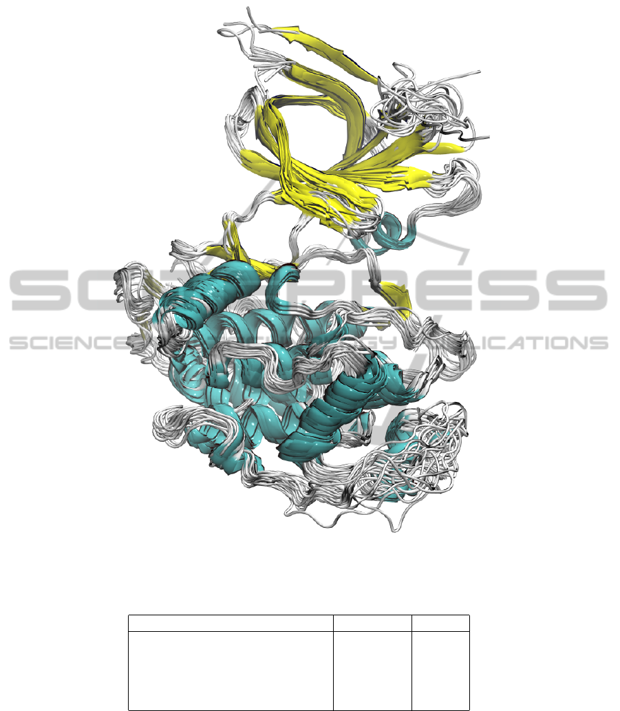
Figure 2: Structural superposition of the 22 PDB entries employed in this study. The structures are depicted in ribbon and
coloured according to the secondary structure elements.
Table 2: Correlations computed with the Mantel test for the different approaches.
Method Correlation p-value
Single value (-1) 0.708 0.001
Single value (0) 0.240 0.071
Single value (+1) 0.305 0.020
Multi values - mean rule 0.548 0.001
Multi values - weighted mean rule 0.721 0.001
virtual screening effort, a number of molecules are
docked at an enzyme-binding site and their bind-
ing affinities are estimated. Assuming that, for each
molecule, only one pose is taken into account (i.e.
the top scoring one), the final ranked distribution
will reflect the molecular preferences of a given pro-
tein. In fact, different proteins will reward differ-
ent classes of molecules, characterized by specific
physico-chemical features. An extension of this con-
sideration is that different conformations of the same
protein will reward different molecules too. This is
because docking algorithms treat these conformations
as if they were different molecular entities altogether.
In this context, the ranked distribution indirectly de-
scribes the physicochemical characteristics of a pro-
tein. We can think of these as fingerprints, where each
AN INNOVATIVE PROTOCOL FOR COMPARING PROTEIN BINDING SITES VIA ATOMIC GRID MAPS
419
0.1
1I09
1GNG
1H8F
2O5K
1J1B
1J1C
1Q3D
1Q4L
1PYX
3DU8
3F7Z
3F88
1Q3W
3GB2
2JLD
3L1S
1Q5K
1UV5
1Q41
3I4B
1R0E
2OW3
(a)
0.1
1GNG
1I09
2O5K
1H8F
1Q3W
3F88
3DU8
1PYX
1J1B
1J1C
3L1S
1UV5
1Q41
1Q5K
3I4B
1Q4L
2JLD
3GB2
1Q3D
2OW3
1R0E
3F7Z
(b)
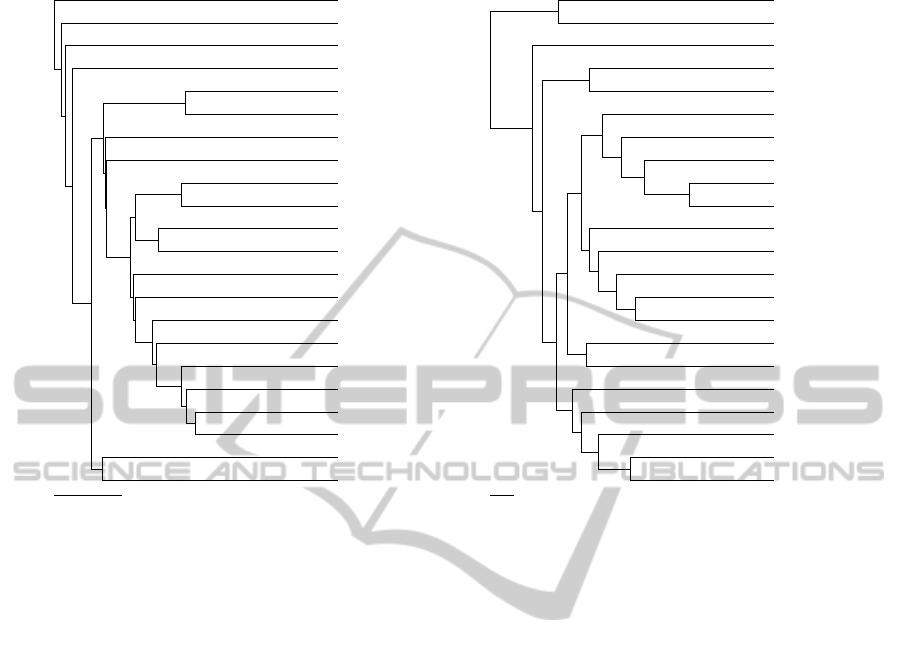
Figure 3: Trees obtained with UPGMA of the phylip package: (a) ground truth; (b) obtained with ’-1’ map.
position in the rank represents a bit and the unique
molecule in that position represents its assigned value.
To obtain meaningful results, a reasonable number
of molecules should be used. The set should be big
enough to allow a fine distinction between proteins,
yet small enough to be computationally feasible. It
should be composed of chemically diverse entries in
order to eliminate noise-generating redundancy. In
this procedure, a set of 6354 diverse compounds was
docked at each of the 22 protein structures. Pear-
sons correlation coefficients calculated between the
obtained ranks represent the final distance, on which
the clustering procedure can be built.
In a real life scenario, where millions of com-
pounds and several tens of proteins can be involved,
using ranked distributions for clustering purposes
could be unfeasible. Grid-driven clustering offers a
quicker approach to this challenge. Moreover, maps-
driven analysis can be more easily interpreted from a
chemical standpoint.
4.2 Quantitative Evaluation
Table 2 reports the correlation coefficients between
the proposed methods and the ground truth distances
(we note that the correlation, in this case, takes val-
ues from -1 to +1 – the higher the value, the better the
result). In addition to the correlation factor, a p-value
is also provided, which measures the probability that
the same correlation is obtained if randomly permut-
ing the rows or the columns of one of the matrices.
Some observations may be drawn from the table:
• the information carried out by the three single-
value maps is rather different: the analysis based
on the single values 0 and +1 is not as good as the
analysis made with the value -1 – even if it shows
a positive correlation with the ground truth
• this is confirmed by the results obtained with the
mean rule (which gives the same weight to all the
maps); a proper weighing of the three distances
yields better results.
• combining the three distances improves the
single-value analysis, thus confirming the com-
plementary information present in the original
sources.
4.3 Qualitative Evaluation
Given the distance, a qualitative analysis could be car-
ried out by looking at trees obtained via the applica-
tion of clustering techniques to the similarity matrices
– the proposed ones and the ground truth ones. In par-
ticular, dendrograms were obtained with the UPGMA
KDIR 2011 - International Conference on Knowledge Discovery and Information Retrieval
420

clustering algorithm (as implemented in the Phylip
Package
2
). In Fig. 3 two trees are reported, namely
the ground truth one and the one obtained with the -1
map.
Rather than looking at the global similarity be-
tween trees, a perceptive comparison should focus
mostly on the local matches. This is because, above a
defined cutoff, distances between entries tend to be
less consistent. Indeed, the map-driven tree repro-
duced nicely some of the trends recorded by the dock-
ing ranks. For instance, entries 1GNG, 1I09, 2O5K
and 1H8F were singletons, according to the ground
truth. As illustrated in Fig. 3, the oxygen map-
driven tree put 5 entries distant from the rest. Four
of those entries were indeed the ground truth single-
tons, while the remaining entry (i.e. 1QW3) was er-
roneously recognized as close to 1H8F. From a bio-
logical perspective, 3 out of those 4 entries were pe-
culiar cases, being the only proteins of the set whose
crystals lacked a molecule bound. Another very inter-
esting achievement is the pairing of 1J1B and 1J1C.
Those Xray structures in fact showed very similar
molecules bound, which in turn yielded highly com-
parable conformational rearrangements. Another no-
table result was found for the cluster composed of
entries 3L1S, 1UV5, 1Q41, 1Q5K and 314B, which
perfectly matched the one found in the ground truth.
Entries 3F88, 3DU8 and 1PYX clustered together in
the map-driven tree. The same trend was found in the
ground truth, with the exception of entry 3F7Z, which
was missing in the former. Overall, the remarkable
resemblance between the ground truth and the map-
driven trees speaks to the accuracy of the proposed
methodology in finding hidden relevant chemical pat-
terns in protein structures. Nonetheless, there is room
for improvement. For instance, in a less reductionist
approach, more atom probes could be used.
5 CONCLUSIONS
In this paper, we proposed a novel computational ap-
proach to comparing two or more proteins, starting
from a physico-chemical description of their binding
site (atomic grid maps). These maps were prepro-
cessed via a chemically plausible procedure that sim-
plified the data while retaining the relevant informa-
tion. Different alignment-based similarity measures
were proposed based on a rigid registration algorithm.
The proposed approach was tested on a real dataset in-
volving 22 proteins. Retrospective evaluations, both
2
All information on software and models could be found
at http://evolution.gs.washington.edu/phylip.html.
qualitative and quantitative, proved the feasibility of
the method.
ACKNOWLEDGEMENTS
We kindly acknowledge the IIT computational plat-
form initiative for providing computer time. We
thank Grace Fox for editing and proofreading the
manuscript.
REFERENCES
Berman, H., Henrick, K., and Nakamura, H. (2003). An-
nouncing the worldwide protein data bank. Nat Struct
Biol, 10:980.
Besl, P. and McKay, N. (1992). A method for registration
of 3d shapes. IEEE Trans. on Pattern Analysis and
Machine Intelligence, 14:239–256.
Bicego, M., Dellaglio, F., and Felis, G. (2007). Multimodal
phylogeny for taxonomy: Integrating information
from nucleotide and amino acid sequences. J. Bioin-
formatics and Computational Biology, 5(5):1069–
1085.
Bottegoni, G., Rocchia, W., Rueda, M., Abagyan, R., and
Cavalli, A. (2011). Systematic exploitation of multi-
ple receptor conformations for virtual ligand screen-
ing. Plos One. in press.
Chen, Y. and Crippen, G. (2005). A novel approach to struc-
tural alignment using realistic structural and environ-
mental information. Protein Sci, 14:2935–2946.
Chen, Y. and Medioni, G. (1992). Object modeling by reg-
istration of multiple range images. Image Vision Com-
puting, 10:145155.
Duin, R. and Tax, D. (2000). Experiments with classifier
combining rules. In Proc. Workshop on Multiple Clas-
sifier Systems, pages 16–29.
Favia, A. (2011). Theoretical and computational ap-
proaches to ligand-based drug discovery. Frontiers in
Bioscience, 16:1276–1290.
Fred, A. and Jain, A. (2005). Combining multiple
clusterings using evidence accumulation. IEEE
Trans. on Pattern Analysis and Machine Intelligence,
27(6):835–850.
Fumera, G. and Roli, F. (2005). A theoretical and experi-
mental analysis of linear combiners for multiple clas-
sifier systems. IEEE Trans. on Pattern Analysis and
Machine Intelligence, 27(6):942–956.
Hernandez, F., De Barreda, E., Fuster-Matanzo, A., Goni-
Oliver, P., Lucas, J., and Avila, J. (2009). The role of
gsk3 in alzheimer disease. Brain Res Bull, 80:248–
250.
Ho, T., Hull, J., and Stihari, S. (1994). Decision combi-
nation in multiple classifier systems. IEEE Trans. on
Pattern Analysis and Machine Intelligence, 16(1):66–
75.
AN INNOVATIVE PROTOCOL FOR COMPARING PROTEIN BINDING SITES VIA ATOMIC GRID MAPS
421

Holm, L. and Sander, C. (1993). Protein structure compar-
ison by alignment of distance matrices. J Mol Biol,
233:123–138.
IUPAC (1997). Compendium of chemical terminology. (the
”Gold Book”). Online corrected version: (1994) ”Van
der Waals forces”.
Jain, A. and Dubes, R. (1988). Algorithms for clustering
data. Prentice Hall.
Jung, J. and Lee, B. (2000). Protein structure alignment
using environmental profiles. Protein Eng, 13:535–
543.
Kahraman, A. and Thornton, J. (2008). Methods to char-
acterize the structure of enzyme binding sites. In
Schwede, T. and Peitsch, M., editors, Computational
Structural Biology - Methods and Applications, vol-
ume 1, pages 189–221. World Scientific Publishing
Co.
Kawabata, T. (2003). Matras: A program for protein 3d
structure comparison. Nucleic Acids Res, 31:3367–
3369.
Kittler, J., Hatef, M., Duin, R., and Matas, J. (1998). On
combining classifiers. IEEE Trans. on Pattern Analy-
sis and Machine Intelligence, 20(3):226–239.
Kumar, A., Wong, D., Shen, H., and Flynn, P. (2003). Per-
sonal verification using palmprint and hand geome-
try biometric. In Proc. of Int. Conf. on Audio and
Video-based biometric person authentication, pages
668–678.
Lorusso, A., Eggert, D., and Fisher, R. (1997). A compar-
ison of four algorithms for estimating 3-d rigid trans-
formations. Machine Vision Applications, 9:272290.
Mantel, N. (1967). The detection of disease clustering and
a generalized regression approach. Cancer Research,
27(2):209–220.
McLachlan, A. (1982). Rapid comparison of protein struc-
tures. Acta Cryst, A38:871–873.
Melnik, O., Vardi, Y., and Zhang, C.-H. (2004). Mixed
group ranks: Preference and confidence in classifier
combination. IEEE Trans. on Pattern Analysis and
Machine Intelligence, 26(8):973–981.
Morphy, R. and Rankovic, Z. (2006). The physicochemi-
cal challenges of designing multiple ligands. J Med
Chem, 49:4961–4970.
Morris, G., Huey, R., Lindstrom, W., Sanner, M., Belew, R.,
Goodsell, D., and Olson, A. (2009). Autodock4 and
autodocktools4: Automated docking with selective re-
ceptor flexibility. J Comput Chem, 30:2785–2791.
Ross, A. and Jain, A. (2004). Multimodal biometrics: an
overview. In Proc. of European Signal Processing
Conference, pages 1221–1224.
Shindyalov, I. and Bourne, P. (1998). Protein struc-
ture alignment by incremental combinatorial exten-
sion (ce) of the optimal path. Protein Eng., 11:739–
747.
Tax, D., Breukelen, M., Duin, R., and Kittler, J. (2000).
Combining classifiers by averaging or by multiplying?
Pattern Recognition, 33:1475–1485.
Topchy, A., Jain, A., and Punch, W. (2005). Clustering en-
sembles: models of consensus and weak partitions.
IEEE Trans. on Pattern Analysis and Machine Intel-
ligence, 27(12):1866–1881.
Totrov, M. (2011). Ligand binding site superposition and
comparison based on atomic property fields: identi-
fication of distant homologues, convergent evolution
and pdb-wide clustering of binding sites. BMC Bioin-
formatics, 12(Suppl 1):S35.
Trucco, E. and Verri, A. (1998). Introductory Techniques
for 3-D Computer Vision. Prentice-Hall.
KDIR 2011 - International Conference on Knowledge Discovery and Information Retrieval
422
