MULTI-FIDELITY DESIGN OPTIMIZATION OF

AXISYMMETRIC BODIES IN INCOMPRESSIBLE FLOW

Leifur Leifsson, Slawomir Koziel and Stanislav Ogurtsov

Engineering Optimization & Modeling Center, School of Science and Engineering, Reykjavik University

Menntavegur 1, 101 Reykjavik, Iceland

Keywords: Axisymmetric body, Underwater vehicles, Hydrodynamic shape optimization, CFD, Direct design, Inverse

design, Surrogate modelling.

Abstract: The paper discusses multi-fidelity design optimization of axisymmetric bodies in incompressible fluid flow.

The algorithm uses a computationally cheap low-fidelity model to construct a surrogate of an accurate but

CPU-intensive high-fidelity model. The low-fidelity model is based on the same governing equations as the

high-fidelity one, but exploits coarser discretization and relaxed convergence criteria. The low-fidelity model is

corrected by aligning the hull surface pressure and skin friction distributions with the corresponding

distributions of the high-fidelity model using a multiplicative response correction. Our approach can be

implemented in both direct and inverse design approaches. Results of two case studies for hull drag

minimization and target pressure distribution matching show that optimized designs are obtained at

substantially lower computational cost (over 94%) when compared to the direct high-fidelity model

optimization.

1 INTRODUCTION

Autonomous underwater vehicles (AUVs) are

becoming increasingly important in various marine

applications, such as oceanography, pipeline

inspection, and mine counter measures (Yamamoto,

2007). Endurance (speed and range) is one of the

more important attribute of AUVs (Allen et al.,

2000). Vehicle drag reduction and/or an increase in

the propulsion system efficiency will translate to a

longer range for a given speed (or the same distance

in a reduced time). A careful hydrodynamic design

of the AUVs, including the hull shape, the

protrutions, and the propulsion system, is therefore

essential.

The fluid flow around an underwater vehicle with

appendages is characterized by flow features such as

thick boundary layers, vortices and turbulent wakes

generated due to the hull and the appendages (Huang

et al., 1992). These flow features can have adverse

effects on, for example, the performance of the

propulsion system and the control planes. Moreover,

the drag depends highly on the vehicle shape, as

well as on the aforementioned flow features. For that

reason, it is important to account for these effects

during the design of the AUVs.

The prediction of the flow past the full three-

dimensional configuration of the AUVs requires the

use of computational fluid dynamics (CFD).

Numerous applications of CFD methods to the flow

past AUVs and other underwater vehicles are in the

literature, e.g., Yang and Löhner, 2003; Barros et al.

2008; and Jagadeesh et al., 2009. The purpose of

these investigations is to predict properties such as

added masses, pressure and friction distributions,

drag, normal force and moment coefficients, wake

field, and stability derivatives. Comparison with

experimental measurements show that CFD is

reliable and can yield accurate results (Yang and

Löhner, 2003; Barros et al. 2008; and Jagadeesh et

al., 2009).

Numerous studies on underwater vehicle design

and optimization have been reported which focus on

the clean hull only, i.e., the appendages and the

propulsion system are neglected and the flow is

taken to be past an axisymmetric body at a zero

angle of attack. Examples of such numerical studies

include Goldschmied (1966), Parsons et al. (1974),

Myring (1976), Dalton and Zedan (1980), Lutz and

Wagner (1998), Alvarez et al. (2009), and Solov’ev

(2009). Allen et al. (2000), however, report an

465

Leifsson L., Koziel S. and Ogurtsov S..

MULTI-FIDELITY DESIGN OPTIMIZATION OF AXISYMMETRIC BODIES IN INCOMPRESSIBLE FLOW.

DOI: 10.5220/0003646104650473

In Proceedings of 1st International Conference on Simulation and Modeling Methodologies, Technologies and Applications (SDDOM-2011), pages

465-473

ISBN: 978-989-8425-78-2

 2011 SCITEPRESS (Science and Technology Publications, Lda.)

experimental investigation of propulsion system

enhancements and drag reduction of an AUV.

The hydrodynamic design optimization of AUVs

in full configuration, taking into account the

appendages and the propulsion system, is still an

open problem. One of the main challenges involved

is the high computational cost of a CFD simulation.

A single CFD simulation of the three-dimensional

flow past an AUV can take a few hours up to several

days, depending on the computational power, the

grid density, and the flow conditions. Therefore, the

direct optimization can be impractial, especially

using traditional gradient-based methods.

An important research area in the field of

aerodynamic optimization is focused on employing

the surrogate-based optimization (SBO) techniques

(Queipo et al., 2005; Forrester and Keane, 2009).

One of the major objectives is to reduce the number

of high-fidelity model evaluations, and thereby

making the optimization process more efficient. In

SBO, the accurate, but computationally expensive,

high-fidelity CFD simulations are replaced—in the

optimization process—by a cheap surrogate model.

SBO has been successfully applied to the

aerodynamic design optimization of various

aerospace components, such as airfoils (e.g.,

Leifsson and Koziel, 2010), aircraft wings (e.g.,

Alexandrov et al., 2000), and turbine blades (e.g.,

Braembussche, 2008).

The surrogate models can be created either by

approximating the sampled high-fidelity model data

using regression (so-called function approximation

surrogates) (see for example Queipo et al., 2005), or

by correcting physics-based low-fidelity models

which are less accurate but computationally cheap

representations of the high-fidelity models (see, e.g.,

Bandler et al., 2004, Alexandrov et al., 2000). The

latter models are typically more expensive to

evaluate. However, less high-fidelity model data is

normally needed to obtain a given accuracy level.

SBO with physics-based low-fidelity models is

called multi- or variable-fidelity optimization.

In this paper, we present a hydrodynamic shape

optimization methodology based on the SBO

concept for AUVs. In particular, we adopt the multi-

fidelity approach with the high-fidelity model based

on the Reynolds-Averaged Navier-Stokes (RANS)

equations, and the low-fidelity model based on the

same equations, but with coarse discretization and

relaxed convergence criteria. We use a simple

response correction to create the surrogate. Here, we

choose to focus on the clean hull design, which is a

convenient case study to implement and test our

design approach.

2 PROBLEM FORMULATION

We constrain the hull shapes to the most common

AUV shape, namely, the torpedo shape, i.e., a three

section axisymmetric body with a nose, a cylindrical

midsection, and a tail. Typically, equipment such as

the computer, sensors, electronics, batteries, and

payload are housed in the nose and the midsection,

whereas the propulsion system is in the tail. Figure 1

shows a typical torpedo shaped hull with a nose of

length a, midsection of length b, overall length L,

and maximum diameter of D.

2.1 Shape Parameterization

We parameterize the nose and the tail using Bézier

curves (Lepine et al., 2001). The Bézier curve, of

degree n, is defined as

∑∑

−

iin

iPktkt

ini

)()())(1(

!)(!

)(

, (1)

where P

, i = 0…n, are the control points, and t is an

× m array from 0 to 1.

We use five control points for the nose and four

for the tail, as shown in Fig. 2. Control points

number three and eight are free (x- and y-

coordinates), while the other points are fixed. We,

therefore, have two design variables for the nose and

tail curves, a total of four design variables, aside

from the hull dimensions a, b, L, and D.

Figure 1: A sketch of a typical axisymmetric torpedo

shaped hull form.

2.2 Design Approaches

The goal of hydrodynamic shape optimization is to

find an optimal—with respect to given objectives—

hull shape, so that given design constraints are

satisfied. There are two main approaches two this

problem. One is to adjust the hull geometrical shape

to maximize performance. This is called direct

design, and the most common design goal, when

considering the clean hull, is drag minimization. An

alternative approach is to define a priori a specific

flow behavior that is to be attained. This is called

inverse design, and, typically in hydrodynamic

design, a target velocity distribution is prescribed

SIMULTECH 2011 - 1st International Conference on Simulation and Modeling Methodologies, Technologies and

Applications

466

(a)

(b)

Figure 2: Bézier curves are used to represent the shapes of

(a) the nose (5 control points); and (b) the tail (4 control

points). Control points 3 and 8 are free, while the other

points are essentially fixed (depend on L, a, b, and D).

(Dalton and Zedan, 1980). Instead, a target pressure

distribution can be prescribed a priori, which is more

common in aerodynamic design (Dulikravich, 1991).

Typically, inverse design minimizes the norm of the

difference between the target and design

distributions. The main difficulty in this approach is

to define the target distribution. In this paper we

consider both the direct and the inverse design

approaches.

3 COMPUTATIONAL MODELS

3.1 High-Fidelity CFD Model

The flow past the hull is considered to be steady and

incompressible. The Reynolds-Averaged Navier-

Stokes (RANS) equations are assumed as the

governing flow equations with the two-equation k-

turbulence model with standard wall functions

(Tannehill et al., 1997).

The solution domain is axisymmetric around the

hull centreline axis and extends two body lengths in

front of the hull, five body lengths behind it, and two

body lengths above it (Fig. 3). At the inlet, there is a

velocity boundary condition where the velocity is set

parallel to the hull axis, i.e., zero angle of attack.

Pressure is prescribed at the outlet (zero gauge

pressure).

Figure 3: The computational solution domain and the

boundary conditions.

The CFD computer code FLUENT (2006) is used

for numerical simulations of the fluid flow.

Asymptotic convergence to a steady state solution is

obtained for each case. The iterative convergence of

each solution is examined by monitoring the overall

residual, which is the sum (over all the cells in the

computational domain) of the L

norm of all the

governing equations solved in each cell. In addition

to this, the drag force (defined in Section 3.3) is

monitored for convergence. A solution is considered

converged if a residual value of 10

-6

has been

reached for all equations, or the number of iterations

reaches 1000.

(a)

(b)

Figure 4: Grid convergence study at a speed of 2 m/s and

Reynolds number of 2 million; (a) the change in the drag

coefficient C

(defined in Section 3.3) with the number of

elements; (b) the variation in the simulation time with

number of elements.

0 0.05 0.1 0.15 0.2

0.02

0.04

0.06

0.08

0.1

x/L

r/L

0.8 0.85 0.9 0.95 1

0.02

0.04

0.06

0.08

0.1

x/L

r/L

0.05

0.1

0.15

0.2

Number of Elements

100

200

300

400

500

600

Number of Elements

Simulation Time [s]

MULTI-FIDELITY DESIGN OPTIMIZATION OF AXISYMMETRIC BODIES IN INCOMPRESSIBLE FLOW

467

The computational grid is structured with

quadrilateral elements. The elements are clustered

around the body and grow in size with distance from

the body. The grids are generated using ICEM CFD

(2006). A grid convergence study was performed to

determine the necessary grid density (Fig. 4). A

torpedo shaped body with L/D = 5 was used in the

study. The inlet speed was 2 m/s and the Reynolds

number was 2 million. Clearly, the drag coefficient

value has converged at the finest grids (number 1

and 2) (Fig. 4(a)). There is, however, a large

difference in the simulation time between the two

finest grids (Fig. 4(b)). Therefore, we selected grid

number 2, with 42,763 elements, to use for the high-

fidelity CFD model in the optimization process.

The velocity contours, pressure and skin friction

distributions are shown in Figs. 5 and 6 for

illustration purposes.

Figure 5: Velocity contours of the flow past an

axisymmetric torpedo shape hull at 2 m/s and Reynolds

number of 2 million. Grid 5 of Fig. 4 was used in the

simulation.

(a)

(b)

Figure 6: Flow distributions (from the high-fidelity and

low-fidelity models (defined in Section 3.2)) on the hull

surface of the flow shown in Fig. 5; (a) the pressure

distribution; and (b) the skin friction distribution.

3.2 Low-Fidelity CFD Model

The low-fidelity model is based on the same CFD

model as the high-fidelity one. However, as the low-

fidelity model will be used in place of the high-

fidelity model in the optimization process, it needs

to be faster than the high-fidelity one. The

simulation time is substantially reduced by making

the grid coarser (Fig. 4(b)). Grid number 6 needs the

lowest simulation time and is the least accurate. A

closer look at that grid reveals that it is too coarse

(the responses were too “grainy”). Consequently, we

selected grid number 5, with 504 elements, to be

used for the low-fidelity model.

The simulation time can be reduced further by

reducing the number of iterations. Figure 7 shows

how the drag coefficient reaches a converged value

after approximately 50 iterations. We therefore relax

the convergence criteria for the low-fidelity model

by setting it to 50 iterations. The ratio of simulation

time of the high-fidelity model to the low-fidelity

model is around 15.

Figure 7: Variation of the drag coefficient with number of

iterations for the case shown in Fig. 5.

3.3 Hull Drag Calculation

For a body in incompressible flow, the total drag is

due to pressure and friction forces, which are

calculated by integrating the pressure (C

) and skin

friction (C

) distributions over the hull surface. The

pressure coefficient is defined as C

≡ (p-p

∞

)/q

∞

where p is the local static pressure, p

∞

is free-stream

static pressure, and q

∞

= (1/2

∞

) is the dynamic

pressure, with

∞

as the free-stream density, and the

∞

free-stream velocity. The skin friction coefficient

is defined as C

≡

∞

, where

is the shear stress.

Typical C

and C

distributions are shown in Fig. 6.

The total drag coefficient is defined as

≡ d/(q

∞

S), where d is the total drag force, and S is

the reference area. Here, we use the frontal-area of

the hull as the reference area. The drag coefficient is

the sum of the pressure and friction drag, or

x/L

r/L

-0.2 0 0.2 0.4 0.6 0.8 1 1.2

0.2

0.4

2.2

2.0

1.8

1.6

1.4

1.2

1.0

0.8

0.6

0.4

0.2

Velocity [m/s]

0 0.2 0.4 0.6 0.8 1

-0.5

0.5

x/L

High-fidelity model

Low-fidelity model

0 0.2 0.4 0.6 0.8 1

0.002

0.004

0.006

0.008

0.01

x/L

0 20 40 60 80 100

0.05

0.1

0.15

0.2

0.25

Iterations

SIMULTECH 2011 - 1st International Conference on Simulation and Modeling Methodologies, Technologies and

Applications

468

DfDpD

CCC +=

, (2)

where C

is the pressure drag coefficient and C

the skin friction drag coefficient. The CFD analysis

yields static pressure and wall shear stress values

(which are non-dimensionalized to give C

and C

) at

the element nodes (Fig. 8). The pressure acts normal

to the surface and the shear stress parallel to it. The

pressure drag coefficient is calculated by integrating

from the leading-edge of the nose to the trailing-

edge of the tail

∫

pDp

dxxrxxCC

)()(sin)(2

θπ

, (3)

where C

(x) is assumed to vary linear between the

element nodes,

(x) is angle of each element relative

to the x-axis, and L is the length of the hull.

Similarly, the skin friction drag coefficient is

calculated as

∫

fDf

dxxrxxCC

)()(cos)(2

θπ

. (4)

4 OPTIMIZATION PROCEDURE

4.1 Design Problem Formulation

Our design task is formulated as a nonlinear

minimization problem of the form

arg min ( )

≤≤

lxu

(5)

where f(

x) is the objective function, x is the design

variable vector, whereas

l and u are the lower and

upper bounds, respectively. Here, no nonlinear

constraints are present, the design variables are control

parameters that parameterize the hull shape (cf. Section

2.1). The objective function depends on the particular

design scenario. For direct design (see Section 2.2), the

objective function is just a drag coefficient as defined

in Section 3.3. For inverse design (see Section 2.2), the

objective is defined as a norm of the difference

between the current and the target pressure

distributions.

4.2 Surrogate-based Optimization

The high-fidelity model evaluation is CPU-intensive

so that solving the problem (5) directly, by plugging

in the high-fidelity model into the optimization loop,

may be impractical. Instead, we would like to

exploit surrogate-based optimization (SBO)

(Bandler et al., 2004; Queipo et al., 2005) that shifts

the optimization burden into the computationally

cheap surrogate, and, thus, allows us to solve (5) at a

low computational cost.

Figure 8: Edge of an element on the hull surface at radius

r. The element length is

Δx and it makes an angle

to the

x-axis. Pressure p acts normal to the hull surface. Shear

stress

acts parallel to the surface.

The generic SBO optimization scheme is the

following

(1) ()

arg min ( )

(6)

where

(i)

, i = 0, 1, ..., is a sequence of approximate

solutions to (5), whereas s

(i)

is the surrogate model at

iteration i. If the surrogate model is sufficiently good

representation of the high-fidelity model f, the

number of iterations required to find a satisfactory

design is small (Koziel et al., 2006).

The surrogate model can be constructed either

from sampled high-fidelity model data using an

appropriate approximation technique (Simpson et

al., 2001), or by utilizing a physically-based low-

fidelity model (Bandler et al., 2004). Here, we

exploit the latter approach as we have a reliable low-

fidelity model at our disposal (see Section 3.2).

Also, good physically-based surrogates can be

constructed using a fraction of high-fidelity model

data necessary to build accurate approximation

models (Koziel and Bandler, 2010a).

There are several methods of constructing the

surrogate from a physically-based low-fidelity

model. They include, among others, space mapping

(SM) (Bandler et al., 2004), various response

correction techniques (Søndergaard, 2003), manifold

mapping (Echeverría and Hemker, 2008), and shape-

preserving response prediction (Koziel, 2010b). In

this paper, the surrogate model is created using a

simple multiplicative response correction, which

turns out to be sufficient for our purposes. An

advantage of such an approach is that the surrogate

is constructed using a single high-fidelity model

evaluation, and it is very easy to implement.

4.3 Surrogate Model Construction

Recall that C

p.f

(x) and C

f.f

(x) denote the pressure and

MULTI-FIDELITY DESIGN OPTIMIZATION OF AXISYMMETRIC BODIES IN INCOMPRESSIBLE FLOW

469

skin friction distributions of the high-fidelity model.

The respective distributions of the low-fidelity model

are denoted as C

p.c

(x) and C

f.c

(x). We will use the

notation C

p.f

(x) = [C

p.f.1

(x) C

p.f.2

(x) ... C

p.f.m

(x)]

, where

p.f.j

(x) is the jth component of C

p.f

(x), with the

components corresponding to different coordinates

along the x/L axis.

At iteration i, the surrogate model C

p.s

(i)

of the

pressure distribution C

p.f

is constructed using the

multiplicative response correction of the form:

() () () ()

...1..2 ..

( ) [ ( ) ( ) ... ( )]

iii iT

ps ps ps psm

CCC C=xxx x

(7)

() ()

.. . ..

() ()

ps j p j pc j

CAC=⋅xx

(8)

j = 1, 2, ..., m, where

() ()

()

() ()

()

pf j

pc j

(9)

Similar definition holds for the skin friction

distribution model C

f.s

(i)

. Note that the formulation

(7)-(9) ensures zero-order consistency (Alexandrov

and Lewis, 2001) between the surrogate and the

high-fidelity model, i.e., C

p.f

(i)

) = C

p.s

(i)

Rigorously speaking, this is not sufficient to ensure the

convergence of the surrogate-based scheme (6) to the

optimal solution of (5). However, because of being

constructed from the physically-based low-fidelity

model, the surrogate (7)-(9) exhibits quite good

generalization capability. As demonstrated in Section

5, this is sufficient for good performance of the

surrogate-based design process.

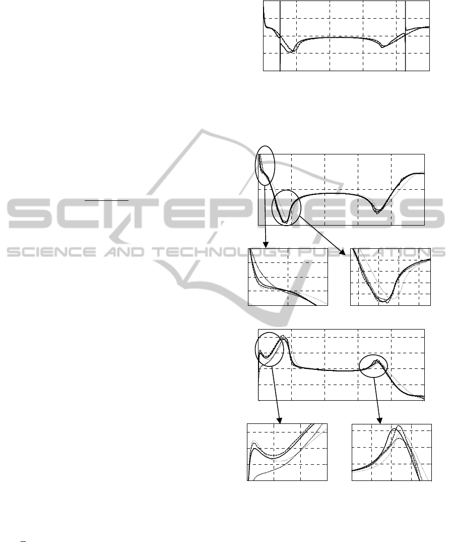
One of the issues of model (7)-(9) is that (9) is not

defined whenever C

p.c.j

(i)

) equals zero, and that the

values of A

p.j

(i)

are very large when C

p.c.j

(i)

) is close to

zero. This may be a source of substantial distortion of

the surrogate model response as illustrated in Fig. 9. In

order to alleviate this problem, the original surrogate

model response is “smoothened” in the vicinity of the

regions where A

p.j

(i)

is large (which indicates the

problems mentioned above). Let j

max

be such that

p.jmax

(i)

| >> 1 assumes (locally) the largest value. Let

Δj be the user-defined index range (typically, Δj =

0.01

⋅m). The original values of A

p.j

(i)

are replaced, for j

= j

max

–Δj, ..., j

max

–1, j

max

, j

max

+1, ..., j

max

+Δj, by the

interpolated values:

max max

()

.max max

max max

() ()

.2 . 1

() ()

.2 . 1

({[ 2 ... 1]

[ 1... 2 ]},

{[ ... ]

[... ]},)

pj j pj j

AIj jj j

jjj j

AA j

−Δ −Δ−

=−Δ−Δ−∪

∪+Δ− +Δ

∪

(10)

Figure 9: Surrogate model C

p.s

(i)

(7)-(9) at x

(i)

(- - -), and at

some other design

x (▬). By definition, C

p.s

(i)

) =

p.f

(i)

). Note that C

p.s

(i)

(x) has large spikes around the

points where C

p.s

(i)

) is close to zero.

(a)

(b)

Figure 10: (a) Smoothened surrogate model (7)-(10)

p.s

(i)

) = C

p.f

(i)

) (—), C

p.s

(i)

(x) (- - -), C

p.c

(x) (⋅ ⋅ ⋅), and

p.s

(x) (▬); (b) Smoothened responses C

f.s

(i)

) = C

f.f

(i)

)

(—), C

f.s

(i)

(x) (- - -), C

f.c

(x) (⋅ ⋅ ⋅), and C

f.s

(x) (▬).

where I(X,Y,Z) is a function that interpolates the

function values Y defined over the domain X onto

the set Z. Here, we use cubic splines. In other words,

the values of A

p.j

(i)

in the neighbourhood of j

max

are

“restored” using the values of A

p.j

(i)

from the

surrounding of j = j

max

–Δj, ..., j

max

+Δj.

0 0.2 0.4 0.6 0.8 1

-1

-0.5

0.5

x/L

0 0.2 0.4 0.6 0.8 1

-0.5

0.5

x/L

0 0.05 0.1

0.2

0.4

0.6

0.8

0.1 0.15 0.2 0.25

-0.5

-0.4

-0.3

-0.2

-0.1

0 0.2 0.4 0.6 0.8 1

0.2

0.4

0.6

0.8

x/L

0 0.05 0.1 0.15

0.4

0.5

0.6

0.7

0.6 0.65 0.7 0.75 0.8

0.35

0.4

0.45

0.5

SIMULTECH 2011 - 1st International Conference on Simulation and Modeling Methodologies, Technologies and

Applications

470

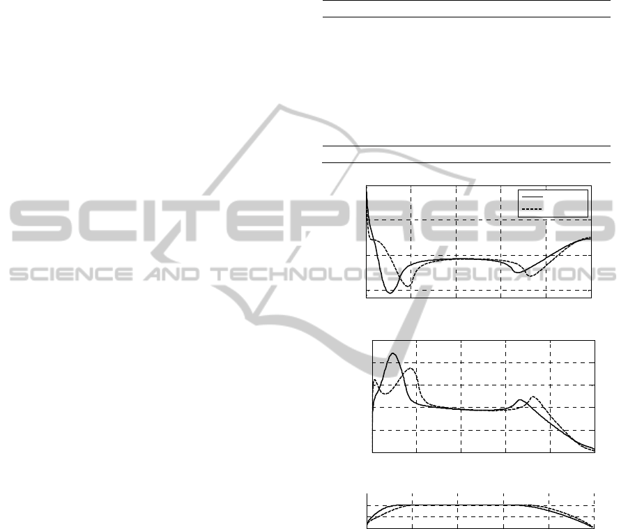
Figure 10(a) shows the “smoothened” surrogate

model response corresponding to that of Fig. 9.

Figure 10 shows the surrogate and the high-fidelity

model responses, both C

and C

, at x

(i)

and at some

other design

5 NUMERICAL EXAMPLES

5.1 General Setup

The proposed approach is applied to the

hydrodynamic shape optimization of torpedo-type

hulls, involving both the direct and inverse design

approaches. Designs are obtained using the

algorithm proposed in Section 4, where the surrogate

model optimization is performed using the pattern-

search algorithm

(Koziel, 2010c). For comparison

purposes, designs obtained through direct

optimization of the high-fidelity model using the

pattern-search algorithm

(Koziel, 2010c) are also

presented.

For both the direct and the inverse design

approaches, the design variable vector is

x = [a x

]

, where a is the nose length, (x

) and (x

)

are the coordinates of the free control points on the

nose and tail Bézier curves, respectively, i.e., points

3 and 8 in Fig. 2. See Section 2.1 for a description of

the shape parameterization. The lower and upper

bounds of design variables are

l = [0 0 0 80 0]

and

u = [30 30 10 100 10]

cm, respectively. Other

geometrical shape parameters are, for both cases, L

= 100 cm, d = 20 cm, and b = 50 cm. The flow speed

is 2 m/s and the Reynolds number is 2 million.

5.2 Direct Design

Numerical results for a direct design case are

presented in Table 1. The hull drag coefficient is

minimized by finding the appropriate shape and

length of the nose and tail sections for a given hull

length, diameter, and cylindrical section length. In

this case, the drag coefficient is reduced by 6.3%.

This drag reduction comes from a reduction in skin

friction and a lower pressure peak where the nose

and tail connect with the midsection (Figs. 11(a) and

11(b)). These changes are due to a more streamlined

nose (longer by 6 cm) and a fuller tail, when

compared to the initial design (Fig. 11(c)).

Table 1: Numerical results for direct drag minimization.

The flow speed is 2 m/s and the Reynolds number is 2

. All the numerical values are from the high-fidelity

model. N

and N

are the number of low- and high-fidelity

model evaluations, respectively.

Variable Initial Pattern-search This work

a 15.0000 21.8611 20.9945

5.0000 5.6758 5.6676

5.0000 2.7022 2.7531

90.0000 98.000 96.6701

5.0000 0.8214 3.0290

0.0915 0.0853 0.0857

N/A 0 300

N/A 282 3

Total cost N/A 282 13

(a)

(b)

(c)

Figure 11: Direct hull drag minimization results showing

initial and optimized (a) pressure distributions; (b) skin

friction distributions; and (c) hull shapes.

The proposed method requires 3 high-fidelity and

300 low-fidelity model evaluations. The ratio of the

high-fidelity model evaluation time to the corrected

low-fidelity model evaluation time varies between

11 to 45, depending on whether the flow solver

converges to the residual limit of 10

-6

, or the

maximum iteration limit of 1000. We express the

total optimization cost of the proposed method in the

equivalent number of high-fidelity model

evaluations. For the sake of simplicity, we use a

0 0.2 0.4 0.6 0.8 1

-0.5

0.5

x/L

Initial

Optimized

0 0.2 0.4 0.6 0.8 1

0.002

0.004

0.006

0.008

0.01

x/L

0 0.2 0.4 0.6 0.8 1

0.05

0.1

r/L

MULTI-FIDELITY DESIGN OPTIMIZATION OF AXISYMMETRIC BODIES IN INCOMPRESSIBLE FLOW

471

fixed value of 30 as the high- to low-fidelity model

evaluation time ratio. The results show that the total

optimization cost of the proposed method is around

13 equivalent high-fidelity model evaluations. The

direct optimization method, using the pattern-search

algorithm (Koziel, 2010c), yields very similar

design, but at the substantially higher computational

cost of 282 high-fidelity model evaluations.

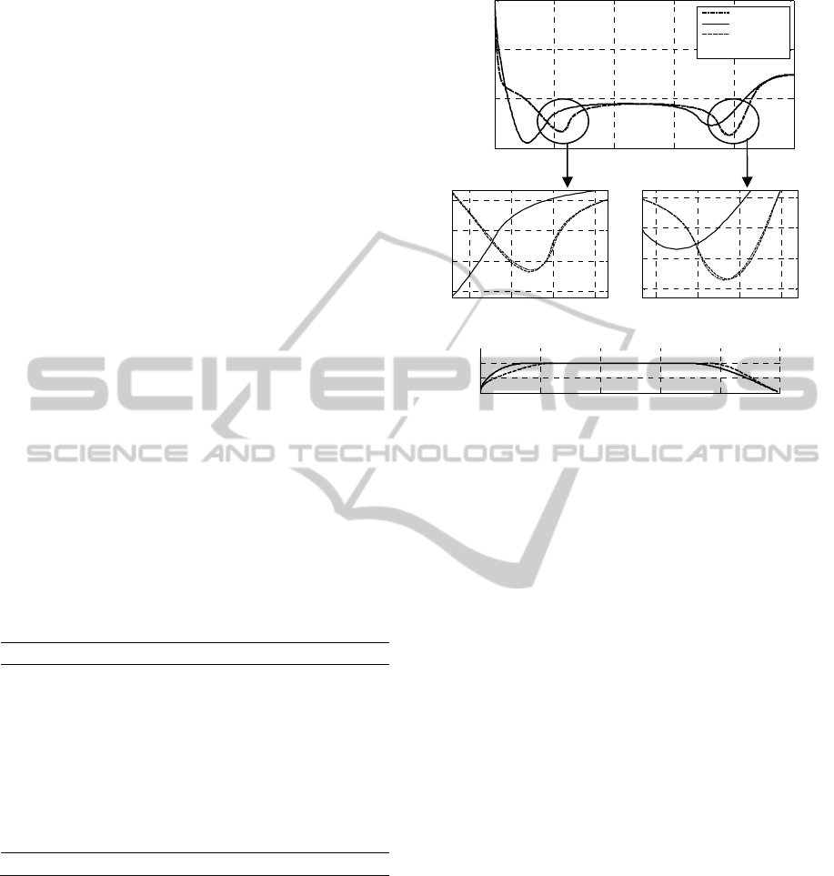
5.3 Inverse Design

Inverse design of the hull shape was performed by

prescribing a target pressure distribution. The

objective is to minimize the norm of the difference

between the pressure distribution of the hull design

and the target pressure distribution. The design

variables and constraints are shown in Section 5.1.

The numerical results are of the inverse design

are presented in Table 2. The proposed algorithm

matched the target pressure distribution (the norm of

the distributions is less than 2

× 10

-5

) using less than

22 equivalent high-fidelity model evaluations. The

direct optimization of the high-fidelity model using

the pattern-search algorithm required 401 function

calls to yield a comparable matching with the target.

Table 2: Numerical results for inverse design optimization

with a target pressure distribution. N

and N

are the

number of low- and high-fidelity model evaluations,

respectively. F is the norm of the difference between the

target and the design shapes.

Variable Initial Pattern-search This work

A 18.000 24.7407 24.7667

7.0000 7.3704 6.8333

8.0000 4.7407 4.5667

85.0000 88.1111 88.6333

7.0000 5.5926 5.3000

F 0.0204 1.64E-5 1.93E-5

0.0925 0.0894 0.0893

N/A 0 500

N/A 401 5

Total cost N/A 401 < 22

6 CONCLUSIONS

Computationally efficient simulation-driven multi-

fidelity design optimization algorithm for

axisymmetric hulls in incompressible fluid flow is

presented. Our algorithm exploits a low-fidelity

model, obtained through a coarse-discretization CFD

simulation, and a response correction method, to

construct a cheap and reliable surrogate of the fluid

(a)

(b)

Figure 12: Results of the inverse design optimization with

a prescribed target pressure distribution; (a) the target,

initial, and optimized pressure distributions; (b) initial and

optimized hull shapes.

flow. The algorithm can be applied to both direct

and inverse design approaches. We demonstrate that

the optimized designs can be obtained at a low

computational cost corresponding to a few high-

fidelity CFD simulations.

REFERENCES

Allen, B., Vorus, W. S., and Prestero, T., 2000, Propulsion

system performance enhancements on REMUS AUVs,

In Proceedings MTS/IEEE Oceans 2000, September,

Providence, Rhode Island.

Alexandrov, N. M., Lewis, R. M., Gumbert, C.R., Green,

L. L., and Newman, P.A., 2000, Optimization with

variable-fidelity models applied to wing design, 38

Aerospace Sciences Meeting & Exhibit, Reno, NV,

AIAA Paper 2000-0841.

Alexandrov, N. M., Lewis, R. M., 2001, An overview of

first-order model management for engineering

optimization. Optimization and Engineering. 2, 413-

430.

Alvarez, A., Bertram, V., and Gualdesi, L., 2009, Hull

hydrodynamic optimization of autonomous

underwater vehicles operating at snorkelling depth,

Ocean Engineering, vol. 36, pp. 105-112.

Bandler, J. W., Cheng, Q. S., Dakroury, S. A., Mohamed,

A. S., Bakr, M.H., Madsen, K., and Søndergaard, J.,

2004, Space Mapping: The State of The Art. IEEE

Trans. Microwave Theory Tech., 52(1), pp. 337-361.

0 0.2 0.4 0.6 0.8 1

-0.5

0.5

x/L

Target

Initial

Optimized

0.15 0.2 0.25 0.3

-0.4

-0.3

-0.2

-0.1

0.7 0.75 0.8 0.85

-0.4

-0.3

-0.2

-0.1

0 0.2 0.4 0.6 0.8 1

0.05

0.1

r/L

SIMULTECH 2011 - 1st International Conference on Simulation and Modeling Methodologies, Technologies and

Applications

472

Braembussche, R. A., 2008, Numerical Optimization for

Advanced Turbomachinery Design, In Optimization

and Computational Fluid Dynamics, Thevenin, D. and

Janiga, G., editors, Springer, pp. 147-189.

Dalton, C., and Zedan, M. F., 1980, Design of low-drag

axisymmetric shapes by the inverse method, J.

Hydronautics, vol. 15, no. 1, pp. 48-54.

Dulikravich, G. S., 1991, Aerodynamic shape design and

optimization, 29

AIAA Aerospace Sciences Meeting,

Reno, NV.

de Barros, E. A., Dantas, J. L. D., Pascoal, A. M., and de

Sá, E., 2008, Investigation of normal force and

moment coefficients for an auv at nonlinear angle of

attack and sideslip angle, IEEE Journal of Oceanic

Engineering, vol. 33, no. 4, pp. 538-549.

Echeverría, D., and Hemker, P.W., 2008, Manifold

mapping: a two-level optimization technique.

Computing and Visualization in Science. 11, pp. 193-

206.

FLUENT, ver. 12.1, ANSYS Inc., Southpointe, 275

Technology Drive, Canonsburg, PA 15317, 2006.

Forrester, A.I.J., and Keane, A.J., 2009, Recent advances

in surrogate-based optimization, Progress in

Aerospace Sciences, vol. 45, no. 1-3, pp. 50-79.

Goldschmied, F.R., 1966, Integrated hull design,

boundary-layer control, and propulsion of submerged

bodies, J. Hydronautics, vol. 1, no. 1, pp. 2-11.

Huang, T. T., Liu, H. L., Groves, N. C., Forlini, T. J.,

Blanton, J. N., and Gowing, S., 1992, Measurements

of flows over an axisymmetric body with various

appendages (DARPA SUBOFF Experiments), In

Proceedings of the 19

Symposium on Naval

Hydrodynamics, Seoul, Korea.

ICEM CFD, ver. 12.1, ANSYS Inc., Southpointe, 275

Technology Drive, Canonsburg, PA 15317, 2006.

Jagadeesh, P., Murali, K., Idichandy, V.G., 2009,

Experimental investigation of hydrodynamic force

coefficients over auv hull form, Ocean Engineering,

vol. 36, pp. 113-118.

Koziel, S., Bandler, J.W., and Madsen, K., 2006, A Space

Mapping Framework for Engineering Optimization:

Theory and Implementation. IEEE Trans. Microwave

Theory Tech., 54(10), pp. 3721-3730.

Koziel, S., and Bandler, J.W., 2010a, Recent advances in

space-mapping-based modeling of microwave devices.

International Journal of Numerical Modelling, (23) 6,

pp. 425-446

Koziel, S., 2010b, Shape-preserving response prediction

for microwave design optimization. IEEE Trans.

Microwave Theory and Tech., 58(11), pp. 2829-2837.

Koziel, S., 2010c, Multi-fidelity multi-grid design

optimization of planar microwave structures with

Sonnet, International Review of Progress in Applied

Computational Electromagnetics, Tampere, Finland,

April 26-29, pp. 719-724.

Leifsson, L., and Koziel, S., 2010, Multi-fidelity design

optimization of transonic airfoils using physics-based

surrogate modeling and shape-preserving response

prediction, Journal of Computational Science, vol. 1,

no. 2, pp. 98-106.

Lepine, J., Guibault, F., Trepanier, J.-Y., and Pepin, F.,

2001, Optimized nonuniform rational b-spline

geometrical representation for aerodynamic design of

wings, AIAA Journal, vol. 39, no. 11, pp. 2033-2041.

Lutz, Th., and Wagner, S., 1998, Numerical shape

optimization of natural laminar flow bodies, In

Proceedings of the 21st ICAS Congress, Sept. 13-18,

Melbourne, Australia.

Myring, D.F., 1976, A theoretical study of body drag in

subcritical axisymmetric flow, Aeronautical

Quarterly, vol. 28, pp. 186-194.

Parsons, J.S., Goodson, R.E., and Goldschmied, F.R.,

1974, Shaping of axisymmetric bodies for minimum

drag in incompressible flow, J. Hydronautics, vol. 8,

no. 3, pp. 100-107.

Queipo, N. V., Haftka, R. T., Shyy, W., Goel, T.,

Vaidynathan, R., and Tucker, P.K., 2005, Surrogate-

Based Analysis and Optimization. Progress in

Aerospace Sciences, 41(1), pp. 1-28.

Simpson, T. W., Peplinski, J., Koch, P.N., Allen, J.K.,

2001, Metamodels for computer-based engineering

design: survey and recommendations. Engineering

with Computers. 17, pp. 129-150.

Solov’ev, S. A., 2009, Determining the shape of an

axisymmetric body in a viscous incompressible flow

on the basis of the pressure distribution on the body

surface, J. of Applied Mechanics and Technical

Physics, vol. 50, no. 6, pp. 927-935.

Søndergaard, J., 2003, Optimization using surrogate

models – by the space mapping technique. Ph.D.

Thesis, Informatics and Mathematical Modelling,

Technical University of Denmark, Lyngby.

Tannehill, J.A., Anderson, D.A., and Pletcher, R.H., 1997,

Computational fluid mechanics and heat transfer, 2

edition, Taylor & Francis.

Yang, C., and Löhener, R., 2003, Prediction of flows over

an axisymmetric body with appendages, The 8

International Conference on Numerical Ship

Hydrodynamics, Sept. 22-25, Busan, Korea.

Yamamoto, I., 2007, Research and development of past,

present, and future auv technologies, in Proc. Int.

Mater-class AUV Technol. Polar Sci. – Soc.

Underwater Technol., Mar. 28-29, pp.17-26.

MULTI-FIDELITY DESIGN OPTIMIZATION OF AXISYMMETRIC BODIES IN INCOMPRESSIBLE FLOW

473