NONLINEAR METAMODELING
AND ROBUST OPTIMIZATION IN AUTOMOTIVE DESIGN
Tanja Clees, Igor Nikitin, Lialia Nikitina and Clemens-August Thole
Fraunhofer Institute for Algorithms and Scientific Computing, Schloss Birlinghoven, 53754, Sankt Augustin, Germany
Keywords: Surrogate models, Bulky data, Multiobjective optimization, Stochastic analysis.
Abstract: We overview the methods for nonlinear metamodeling of a simulation database featuring continuous
exploration of simulation results, tolerance prediction, sensitivity analysis, robust multiobjective
optimization and rapid interpolation of bulky FEM data. Large scatter of simulation results, in crash-test
simulations caused for example by buckling, is still a challenging issue for increasing predictability of
simulation and accuracy of optimization results. For industrially relevant simulations with large scatter,
novel stochastic methods are introduced and their efficiency is demonstrated for benchmark cases.
1 INTRODUCTION
Simulation is an integral component of virtual
product development today. The task of simulation
consists mainly in solution of physical models in the
form of ordinary or partial differential equations.
From the viewpoint of product development the real
purpose is product optimization, and the simulation
is "only" means for the purpose. Optimization means
searching for the best possible product with respect
to multiple objectives (multiobjective optimization),
e.g. total weight, fuel consumption and production
costs, while the simulation provides an evaluation of
objectives for a particular sample of a virtual
product.
The optimization process usually requires a
number of simulation runs, the results form a
simulation dataset. To keep simulation time as short
as possible, "Design of Experiments" (DoE, (Tukey
1997)) is applied, where a space of design variables
is sampled by a limited number of simulations. On
the basis of these samples, a surrogate model is
constructed, e.g. a response surface (Donoho, 2000),
which describes the dependence between design
variables and design objectives. Modern surrogate
models (Jones et al. 1998; Keane et al. 2005; Nikitin
et al. 2008-2010) describe not only the value of a
design objective but also its tolerance limits, which
allow to control precision of the result. Moreover,
not only scalar design objectives but whole
simulation results, even highly resolved in
space/time, (”bulky” dataset) can be modeled
(Nikitin et al., 2008-2010).
In this paper we will concentrate on stochastic
aspects of simulation processes. Industrial
simulations, e.g. virtual crash tests, often possess a
random component, related to physical and
numerical instabilities of the underlying simulation
model and uncertainties of its control parameters.
Under these conditions the user is interested not only
in the mean value of an optimization criterion, e.g.
crash intrusion, but also in its scatter over
simulations. In practice, it is required to fulfil
optimization objectives with a certain confidence,
e.g. 6-sigma. This task belongs to the scope of
robustness or reliability analysis.
Often, the confidence intervals are so large that
one has to reduce scatter before optimization. There
is a part of scatter deterministically related to the
variation of design variables, which can be found by
means of sensitivity analysis. The other part is
purely stochastic. It can be triggered by microscopic
variations of design variables and - even if they are
fixed - by the numerical process itself, e.g. by
random scheduling in multiprocessing simulation.
These microscopic sources are then amplified by
inherent physical instabilities of the model related
e.g. to buckling, contact phenomena or material
failure. Stochastic analysis allows to track the
sources of scatter, to reconstruct causal chains and to
identify hidden parameters describing chaotic
behavior of the model. If uncontrolled, these
parameters propagate scatter to the optimization
483
Clees T., Nikitin I., Nikitina L. and Thole C..
NONLINEAR METAMODELING AND ROBUST OPTIMIZATION IN AUTOMOTIVE DESIGN.
DOI: 10.5220/0003646704830491
In Proceedings of 1st International Conference on Simulation and Modeling Methodologies, Technologies and Applications (SDDOM-2011), pages
483-491
ISBN: 978-989-8425-78-2
Copyright
c
 2011 SCITEPRESS (Science and Technology Publications, Lda.)

objectives. The challenge is to put them under
control, at least partially, e.g. by predeformation of
buckling parts, adjustment of contact conditions,
placement of additional welding points etc. In this
way the scatter of simulation can be suppressed and
optimization becomes more robust.
In Sec.2 we will overview the methods for
metamodeling of bulky simulation results; in Sec.3
we describe stochastic methods for reliability and
causal analysis; Sec.4 presents applications of these
methods to real-life examples in automotive design.
The approaches presented in this paper have been
implemented in software tools DiffCrash (Thole et al
2003-2008) and DesParO (Nikitin et al., 2008-2010)
and have been subjects of international patent
applications (DPMA 10 2009 057295.3 and PCT/
EP2010/061439).
2 RBF METAMODEL
Numerical simulations define a mapping y=f(x):
R
n
→R
m
from n-dimensional space of simulation
parameters to m-dimensional space of simulation
results. In crash test simulation the dimensionality of
simulation parameters x is moderate (n~10-30),
while simulation results y are dynamical fields
sampled on a large grid, typically containing
millions of nodes and hundreds of time steps,
resulting in values of m~10
8
. High computational
complexity of crash test models restricts the number
of simulations available for analysis (typically
Nexp<10
3
) which is preferred to be as small as
possible.
Metamodeling with radial basis functions (RBF)
is a representation of the form
f(x)=∑
i=1.. Nex
p
c
i
Φ
(|x-x
i
|),
(1)
where Φ() are special functions, depending only on
the Euclidean distance between the points x and x
i
.
The coefficients c
i
can be obtained by solving a
linear system
y
i
=∑
j
c
j
Φ(|x
i
-x
j
|)
(2)
where y
i
=f(x
i
). The solution can be found by direct
inversion of the moderately sized Nexp*Nexp
system matrix Φ
ij
=Φ(|x
i
-x
j
|). The result can be
written in a form of weighted sum f(x)=∑
i
w
i
(x)y
i
,
with the weights
w
i
(x)=∑
j
Φ
-1
i
j
Φ(|x-x
j
|).
(3)
A suitable choice for the RBF, providing non-
degeneracy of Φ-matrix for all finite datasets of
distinct points and all dimensions n, is the multi-
quadric function (Buhmann 2003) Φ(r)=(b
2
+r
2
)
1/2
,
where b is a constant defining smoothness of the
function near data point x=x
i
. RBF interpolation can
also be combined with polynomial detrending,
adding a polynomial part p():
f(x)=
∑
i=1..Nex
p
c
i
Φ
(|x-x
i
|)+p(x).
(4)
This allows reconstructing exactly polynomial
(including linear) dependencies and generally
improving precision of interpolation. The precision
can be controlled via the following cross-validation
procedure: the data point is removed, data are
interpolated to this point and compared with the
actual value at this point. For an RBF metamodel
this procedure leads to a direct formula (Nikitin et
al., 2010)
err
i
= f
inter
p
ol
(x
i
)-f
actual
(x
i
) = -c
i
/(Φ
-1
)
ii
.
(5)
Specifics of Bulky Data: although RBF metamodel
is directly applicable for interpolation of
multidimensional data, it contains one matrix-vector
multiplication f(x)=yw(x), comprising O(mNexp)
floating point operations per every interpolation.
Here y
ij
, i=1..m, j=1..Nexp is the data matrix, where
every column forms one experiment, every row
forms a data item varied in experiments.
Dimensional reduction technique applicable for
acceleration of this computation is provided by
principal component analysis (PCA). At first, an
average value is row-wise subtracted, forming
centered data matrix dy
ij
= y
ij
- <y
i
>. For this matrix
a singular value decomposition (SVD) is written:
dy=UΛV
T
, where Λ is a diagonal matrix of size
Nexp*Nexp, U is a column-orthogonal matrix of
size m*Nexp, V an orthogonal square matrix of size
Nexp*Nexp:
U
T
U=1, V
T
V=VV
T
=1. (6)
A computationally efficient method (Nikitin et al
2010) for this decomposition in the case m>>Nexp
is to find Gram matrix G=dy
T
dy, to perform its
spectral decomposition G=VΛ
2
V
T
, and to compute
the remaining U-matrix with post-multiplication
U=dyVΛ
-1
. The Λ values are non-negative and
sorted in non-ascending order. If all these values in
the range k>Nmod are omitted (set to zero), the
resulting reconstruction of y-matrix will have a
deviation δy. L
2
-norm of this deviation gives
err
2
=
∑
i
j
δ
y
i
j
2
=
∑
k>Nmod
Λ
k
2
(7)
(Parseval’s criterion). This formula allows
controlling precision of reconstructed y-matrix.
SIMULTECH 2011 - 1st International Conference on Simulation and Modeling Methodologies, Technologies and
Applications
484

.
Usually Λ
k
rapidly decreases with k, and a few first
Λ values give sufficient precision. The result of
interpolation is represented as a product df=Ψg of
SVD modes Ψ=UΛ (principal components) to SVD-
transformed RBF weights g=V
T
w. Finally one has
f(x)=<y>+df(x), computational cost of interpolation
is reduced to O(m Nmod), plus once-charged O(m
Nexp
2
) cost of SVD. This method is convenient
when interpolation should be performed many times
(>>Nexp), e.g. for interactive exploration of
database.
More generally, for representation of bulky data
one can use clustering techniques (Nikitin et al.,
2010). They also decompose bulky data over a few
basis vectors (modes) and accelerate linear algebra
operations with them.
3 RELIABILITY ANALYSIS
The purpose of reliability analysis is an estimation
of confidence limits (CL) for simulation results:
P(y<CL)=C, where P is probability measure and C is
a user specified confidence level. For example,
median corresponds to 50% CL, i.e. P(y<med)=0.5;
while 68% CL corresponds to confidence interval
[CLmin,CLmax], where P(y<CLmin)=0.16,
P(y≥CLmax)=1-P(y<CLmax)=0.16; etc. Several
methods for solution of this task are available.
3.1 First Order Reliability Method
(FORM)
FORM is applicable for linear mapping f(x) and
normal distribution of simulation parameters:
ρ
(x)~exp(-(x-x
0
)
T
cov
x
-1
(x-x
0
)/2).
(8)
Here x
0
=<x> is mean value of x and
(cov
x
)
i
j
=<(x-x
0
)
i
(x-x
0
)
j
> (9)
is covariance matrix of x. In this case y is also
normally distributed, with mean value
y
0
=<y>=med(y)=f(x
0
(10)
and covariance matrix
cov
y
= J cov
x
J
T
, (11)
where J
ij
= ∂f
i
/∂x
j
is Jacoby matrix of f(x), called
also sensitivity matrix. The diagonal part of cov
y
gives standard deviations σ
y
2
directly defining
CL(y), e.g.
CL
min/max
(68%)=<y>±σ
y
,
(12)
CL
min/max
(99.7%)=<y>±3σ
y
.
(13)
In particular, when simulation parameters are
independent random values, cov
x
becomes diagonal:
cov
x
=diag(σ
x
2
), and
σ
y
i
2
=
∑
j
=1..n
(
∂
f
i
/
∂
x
j
)
2
σ
x
j
2
.
(14)
A finite difference scheme used to compute Jacoby
matrix of f(x) requires Nexp=O(n) simulations, e.g.
2n for central difference scheme plus one
experiment at x
0
, Nexp=2n+1. The algorithm
possesses computational complexity O(nm) and can
be implemented efficiently as reading data from
Nexp simultaneously open data streams and writing
CL to a single output data stream. In this way the
memory requirements can be minimized and
parallelization can be done straightforwardly.
3.2 Second Order Reliability
Method (SORM)
SORM is applicable for slightly non-linear mapping
f(x), which can be approximated by quadratic
functions. The distributions ρ(x) are normal or can
be cast to normal ones by a suitable transformation
of parameter. For quadratic approximations CL can
be explicitly computed (Cizelj et al., 1994) using
main curvatures in the space of normalized variables
z
i
=(x-x
0
)
i
/σ
xi
, i.e. eigenvalues of Hesse matrix
H
i
jk
=∂
2
f
i
/∂z
j
∂z
k
. These eigenvalues can be also used
to estimate non-linearity of the mapping f(z), by
maximizing the 1st and 2nd Taylor's terms over a
ball of radius R:
max
|z|≤R
Jz=|J|R, max
|z|≤R
|z
T
Hz/2|=Hmax R
2
/2,
(15)
so that the linear term prevails over quadratic one, in
this ball, iff |J|>>Hmax R/2. Here
J
ij
=
∂
f
i
/
∂
z
j
, |J|=(
∑
j
J
ij
2
)
1/2
(16)
and Hmax is maximal absolute eigenvalue of H.
Both this criterion and estimation of main curvatures
require full Hesse matrix, i.e. Nexp=O(n
2
)
simulations. Practically, the usability of SORM is
limited, because strongly non-linear functions would
involve higher order terms and because distributions
of simulation parameters can strongly deviate from
normal ones.
3.3 Confidence Limits Determination
with Monte Carlo Method
(CL-MC)
In the case of non-linear mapping f(x) and arbitrary
distribution ρ(x) general Monte Carlo method is
applicable. The method is based on estimation of
probability
NONLINEAR METAMODELING AND ROBUST OPTIMIZATION IN AUTOMOTIVE DESIGN
485

P
N
(y<CL) = num.of (y
n
<CL)/N
(17)
for a finite sample {y
1
,...,y
N
}. By the law of large
numbers (van der Vaart, 1998), F
N
=P
N
(y<CL) is
consistent unbiased estimator for F=P(y<CL), i.e.
F
N
→F with probability 1, when N→∞ and <F
N
> =
F for all finite N. By the central limit theorem (van
der Vaart 1998), the error of such estimation
err
N
=F
N
-F at large N is distributed normally with
zero mean and standard deviation σ∼(F(1-F)/N)
1/2
.
Algorithmically the method consists of three phases:
(CL1) generation of N random points in parameter
space according to user specified distribution ρ(x),
(CL2) numerical simulations for given parameter
values,
(CL3) determination of confidence limits by one-
pass reading of simulation results, sorting m samples
{y
1
,...,y
N
} and selection of k-th item in every sample
with k=[(N-1)F+1] as a representative for CL.
The analysis phase of the algorithm possesses
computational complexity O(mN log N) and can be
efficiently implemented using data stream operations
similar to FORM. Precision of the method is
estimated using standard deviation formula above.
Remarkably, the precision depends neither on
dimension of parameter space n, nor on the length of
simulation result m, but only on sample size
N=Nexp and user-specified confidence level F=C.
For instance, CL determination at the level 68%
(F=0.16) with 4% precision requires Nexp=84, while
for 68%±1% one needs Nexp=1344.
3.4 Monte Carlo Combined with RBF
Metamodel (MC-RBF)
Large sample size is required for precise
determination of CL with Monte Carlo method. To
reduce the number of required simulations, RBF
metamodel can represent the mapping f(x) during
analysis phase of CL-MC. While a metamodel can
be constructed using a moderate number of
simulations, e.g. Nexp~100, determination of CL
can be done with N>>Nexp. Application of RBF
metamodel for CL computation proceeds similarly
to CL-MC. The only difference is that Nexp
parameter points generated at phase (CL1) are used
as input for the metamodel. They should not
necessarily possess user specified distribution, but
one providing better precision of metamodel, i.e.
better covering "the corners" of parameter space. It
is especially important for populating tails of
distribution, corresponding to high confidence e.g.
99.7% CL. Uniform distribution is suitable for this
purpose. Then, after numerical simulations at phase
(CL2), and after filtering out failed experiments, the
actual distribution ρ(x) is used to generate N
parameter points, and construct RBF weight matrix
w
ij
=w
i
(x
j
), i=1..Nexp, j=1..N. This matrix is used in
phase (CL3) for multiplication with simulation
results y
ik
, k=1..m, comprising O(m N Nexp)
operations, which usually prevails over O(m N log
N) operations needed for sorting of interpolated
samples.
4 CAUSAL ANALYSIS
Causal analysis is determination of cause-effect
relationships between events. In context of crash test
analysis, this usually means identification of events
or properties causing the scatter of the results. This
allows to find sources of physical or numerical
instabilities of the system and helps to reduce or
completely eliminate them.
Causal analysis is generally performed by means
of statistical methods, particularly, by estimation of
correlation of events. It is commonly known that
correlation does not imply causation (this logical
error is often referred as "cum hoc ergo propter
hoc": "with this, therefore because of this"). Instead,
strong correlation of two events does mean that they
belong to the same causal chain. Two strongly
correlated events either have direct causal relation or
they have a common cause, i.e. a third event in the
past, triggering these two ones. This common cause
will be revealed, if the whole causal chain i.e. a
complete sequence of causally related events will be
reconstructed. Practical application of causal
analysis requires formal methods for reconstruction
of causal chains.
A practical problem of causal analysis in crash-
test simulations is often not a removal of a prime
cause of scatter, which is the crash event itself. It is
more an observation of propagation paths of the
scatter, with a purpose to prevent this propagation,
by finding regions where scatter is amplified (e.g.
break of a welding point, pillar buckling, slipping of
two contact surfaces etc). Since a small cause can
have large effect, formally earliest events in the
causal chain can have a microscopic amplitude
("butterfly effect"). Therefore it is reasonable to
search for amplifying factors and try to eliminate
them, not the microscopic sources.
As input for causal analysis the centered data
matrix dy
ij
, i=1..m, j=1..Nexp is used. Here every
column forms one experiment, every row forms a
data item varied in experiments, and the mean value
SIMULTECH 2011 - 1st International Conference on Simulation and Modeling Methodologies, Technologies and
Applications
486

.
<y> is row-wise subtracted from the matrix. Then
every data item is transformed to a z-score vector
(Larsen and Marx, 2001):
z
ij
=dy
ij
/|dy
i
|, |dy
i
|=sqrt(∑
j
dy
ij
2
),
(18)
or by means of the equivalent alternative formula
z
ij
=dy
ij
/(s(y
i
)(N
exp
)
1/2
), s(y
i
)=(∑
j
dy
ij
2
/N
exp
)
1/2
.
(19)
Here s(y
i
) is the root mean square deviation of the i-
th data item, which can serve as a measure of scatter.
In this way the data items are transformed to m
vectors in Nexp-dimensional space. All these z-
vectors belong to an (Nexp-2)-dimensional unit-
norm sphere, formed by intersection of a sphere
|z|=1 with a hyperplane ∑
j
z
ij
=0. The scalar product
of two z-vectors is equal to Pearson's correlator of
data items:
(z
1
,z
2
) = ∑
j
z
1j
z
2j
= corr(y
1
,y
2
).
(20)
An important role of this representation is the
following. Strongly correlated data items correspond
either to coincident (z
1
=z
2
) or opposite (z
1
=-z
2
) z-
vectors. If not the sign but only the fact of
dependence is of interest, one can glue opposite
points together formally considering a sphere of z-
vectors as projective space. Using this
representation, one can apply (Nikitin et al., 2010)
general purpose clustering methods such as k-means
to group data items distributed on this sphere to a
few strongly correlated components.
In spite of their numerical efficiency, these
clustering methods neglect temporal ordering of
events, while in causal analysis the task is to find an
earliest physically significant event in the causal
chain. In crash test simulation such events
correspond to bifurcation points, where the scatter
appears "ex nihilo". Such points are clearly visible
as spikes in dynamical scatter plots s(y), the problem
is that there are too many of them. Although
decision between potential candidates by a formal
algorithm can be difficult, an engineering knowledge
allows to narrow the search to significant parts
where scatter propagation can be really initiated by
physical effects, such as buckling of longitudinal,
break of welding point etc. The other problem is that
in bifurcation points new scatter is just appeared and
it is generally hidden under the consequences of
previous effects. At first one needs to separate
scatter contributions.
Considering two data items dy(a) and dy(b), one
can define contribution relevant to the data item (a)
in (b) as follows:
dy|
a
(b) = corr(a,b)s(b)z(a).
(21)
After subtraction of this contribution a residual
dy(b)-dy|
a
(b) does not correlate with dy(a), and the
scatter does not increase.
s
2
|
a
(b)=<(dy(b)-dy|
a
(b))
2
>=s
2
(b)(1-corr
2
(a,b))
(22)
Armed with this subtraction procedure, we
propose the following algorithm for causal analysis.
Temporal Clustering:
(T1) visualize scatter state-by-state;
(T2) isolate bifurcation point;
(T3) subtract its contribution from the scatter in
consequent states;
(T4) if scatter is still remaining, goto (T1).
Here subtraction of scatter from previous
bifurcations reveals new bifurcations hidden under
the consequences of previous ones. The remaining
scatter monotonously falls during the iterations, and
the iterations can be stopped when the scatter
becomes small everywhere or in the regions of
interest.
The geometrical meaning of subtraction
procedure: b-b|
a
=b-(a,b)/(a,a)a is an orthogonal
projection in the space of data items and the whole
sequence is Gram-Schmidt (GS) orthonormalization
procedure applied in the order of appearance of
bifurcation points a
i
. The obtained orthonormal basis
g
i
=GS(a
i
) can be used for reconstruction of all data
by the formula:
dy=
∑
i
Ψ
i
g
i
+res,
Ψ
i
=(dyg
i
).
(23)
The norm of residual is controlled by remaining
scatter, which is small according to our stop
criterion:
|res|
2
/Nexp=s
⊥
2
(y)=s
2
(y)-∑
i
Ψ
i
2
/Nexp.
(24)
Algorithmically every i-th iteration one computes a
scalar field Ψ
i
describing contribution of i-th
bifurcation point to scatter of the model and a scalar
field s
i⊥
2
(y) used for determination of the next
bifurcation point a
i+1
, or for stop criterion
s
i⊥
2
(y)<threshold. This requires O(mNexp) floating
point operations per iteration.
Matrix decomposition of the form dy=Ψg is
similar to PCA described above, with the other
meaning of the modes Ψ. Like in PCA, Ψ are scalar
fields distributed over dynamical model which are
common for all experiments. They have the other
temporal profile than PCA modes, reflecting causal
structure of scatter: they start at corresponding
bifurcation points and propagate forward in time.
Differently from PCA modes, they are not
orthogonal columnwise, i.e. with respect to scalar
product over the model. g-coefficients form
NONLINEAR METAMODELING AND ROBUST OPTIMIZATION IN AUTOMOTIVE DESIGN
487

Nexp*Nmod columnwise orthonormal matrix. Like
corresponding matrix in PCA, they define an
orthonormal basis in the space of experiments, with
respect to the scalar product coincident with
Pearson's correlator.
The scatter associated with design variables can
be treated by the same method, if one puts data items
containing variation of design variables as the first
candidates for bifurcation points. The corresponding
Ψ-modes will represent sensitivities of simulation
results to variation of parameters. The remaining
scatter represents indeterministic part of the
dependence. The corresponding Ψ-modes are
bifurcation profiles and their g-coefficients are those
hidden variables which govern purely stochastic
behavior of the model. One can either take hidden
variables into account when performing reliability
analysis, or try to put them under control for
reducing scatter of the model.
5 EXAMPLES
5.1 Audi B-pillar Crash Test
The model shown on Fig.1 contains 10 thousand
nodes, 45 timesteps, 101 simulations. Two
parameters are varied representing thicknesses of
two layers composing a part of a B-pillar. The
purpose is to find a Pareto-optimal combination of
parameters simultaneously minimizing the total
mass of the part and crash intrusion in the contact
area. To solve this problem, we have applied the
methods described in Sec.2, namely RBF
metamodeling of target criteria for multiobjective
optimization and PCA for compact representation of
bulky data. Based on these methods, our interactive
optimization tool DesParO supports real-time
interpolation of bulky data, with response times in
the range of milliseconds. As a result, the user can
interactively change parameter values and
immediately see variations of complete simulation
result, even on an ordinary laptop computer.
In more details, Fig.1 shows the optimization
problem loaded in the Metamodel Explorer, where
design variables (thicknesses1,2) are presented at the
left and design objectives (intrusion and mass) at the
right. First, the user imposes constraints on design
objectives, trying to minimize intrusion and mass
simultaneously, as indicated by red ovals on Fig.1
(upper part). As a result, “islands” of available
solutions become visible along the axes of design
variables. Exploration of these islands by moving
corresponding sliders shows that there are two
optimal configurations, related cross-like, as
indicated on Fig.1 (middle). For these
configurations, both constraints on mass and
intrusion are satisfied, while they correspond to
physically different solutions, distinguished by an
auxiliary velocity criterion. For every criterion also
its tolerance is shown corresponding to 1-sigma
confidence limits, as indicated by horizontal bars
under the corresponding slider as well as +/- errors
in the value box. This indication allows satisfying
constraints with 3-sigma (99.7%) confidence, as
shown on the images. The Geometry Viewer, shown
at the bottom of Fig.1, allows to inspect the optimal
design in full details. E.g. on the two images at the
bottom, one can see the difference between small
and large thickness values resulting in softer or
stiffer crash behavior.
While performing constraint optimization, the
user immediately sees how small mass solutions
disappear when intrusion is minimized. This gives
an intuitive feeling for the trade-off (Pareto
behavior) between optimization objectives. With
these capabilities and complementary information
such as auxiliary criteria and interactive
interpolation of bulky simulation results, “the”
optimal solution, i.e. a single representative on the
Pareto front, can be selected by a user decision.
5.2 Ford Taurus Crash Test
The crash model shown on Fig.2 contains 1 million
nodes, 32 timesteps, 25 simulations. Processing of
this model with the temporal clustering algorithm
described above has been performed on a 16-CPU
Intel-Xeon 2.9GHz workstation with 24GB main
memory. It required 3min per iteration and
converged in 4 iterations.
Crash intrusions in the foot room of the driver
and passenger are commonly considered as critical
safety characteristics of car design. These
characteristics possess numerical uncertainties, the
analysis of which falls in the subject of Sec.3-4. The
upper left part of Fig.2 shows the scatter measure
s(y), in mm, distributed on the model. The scatter in
the foot room is so large (>10mm) that direct
minimization of intrusion is impossible. Temporal
clustering allows to identify sources of this scatter
and subtract relevant contributions. Further images
show how the scatter decreases in these subtractions.
After the 4
th
iteration the scatter in the foot room
reaches a safe level (<3mm). Several bifurcation
points have been identified and subtracted per
iteration; in this way the performance of the
algorithm has been optimized. The two major
SIMULTECH 2011 - 1st International Conference on Simulation and Modeling Methodologies, Technologies and
Applications
488

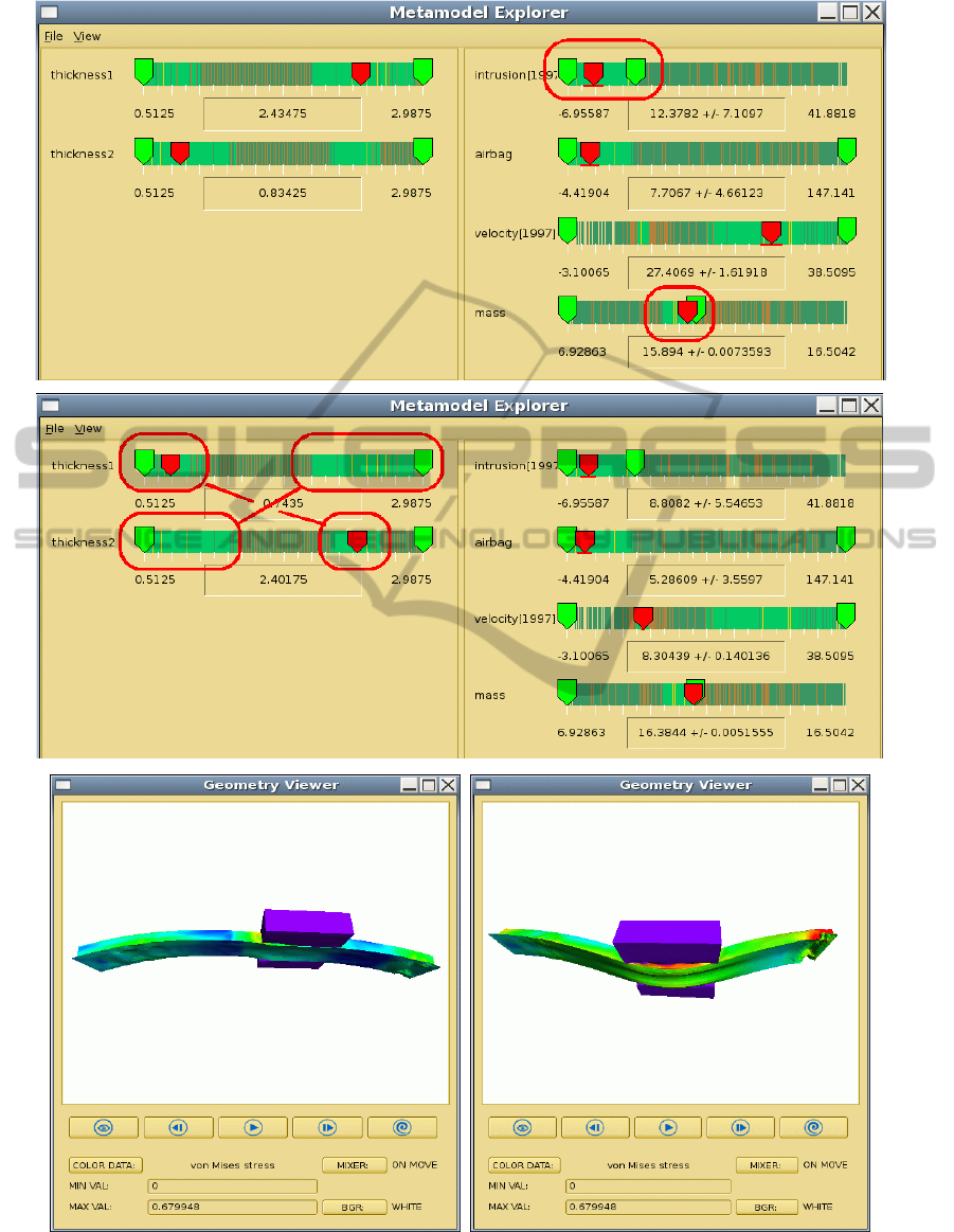
Figure 1: Audi B-Pillar crash test in DesParO Metamodel Explorer. Top: constraints on intrusion and mass are imposed.
Center: two optimal designs are found. Bottom: inspection of optimal design in DesParO Geometry Viewer.
NONLINEAR METAMODELING AND ROBUST OPTIMIZATION IN AUTOMOTIVE DESIGN
489

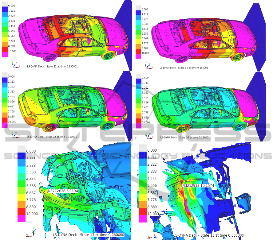
Figure 2: Temporal clustering of Ford Taurus crash test using DiffCrash. Upper left: original scatter in mm. Upper right –
center left – center right: consequent iterations of scatter subtraction. Bottom: two major bifurcations found.
bifurcations found are shown on the bottom part of
Fig.2. They represent buckling phenomena on the
left longitudinal rail and a fold on the floor of the
vehicle, which appear in earlier time steps. In total,
15 bifurcation points have been identified,
representing statistically independent sources of
scatter. The whole scatter in the model can be
decomposed over the corresponding basis functions
Ψ(y). In this way the dimensionality of the problem
is reduced to 15 variables (g-coefficients)
completely describing the stochastic behavior of the
model.
6 CONCLUSIONS
We have presented and discussed methods for
nonlinear metamodeling of a simulation database
featuring continuous exploration of simulation
results, tolerance prediction and rapid interpolation
of bulky FEM data. For the purpose of robust
optimization, the approach has been extended by the
methods of reliability and causal analysis. The
efficiency of the methods has been demonstrated for
several application cases from automotive industry.
Further plans include to use the results of causal
analysis as a basis for modifications of a simulation
model for improving its stability. We also plan to
consider non-linear relationships between stochastic
variables. Linear methods such as PCA and GS
SIMULTECH 2011 - 1st International Conference on Simulation and Modeling Methodologies, Technologies and
Applications
490

.
determine only a linear span over principal
components, while some stochastic variables can
become non-linear functions of others. For
determination of such dependencies the methods of
curvilinear component analysis (CCA) can be
applied.
ACKNOWLEDGEMENTS
Many thanks to the team of Prof. Steve Kan at the
NCAC and the Ford company for providing the
publically available LS-DYNA models and to
Andreas Hoppe and Josef Reicheneder at AUDI for
providing PamCrash B-pillar model. The availability
of these models fosters method developments for
crash simulation. We are also grateful to Michael
Taeschner and Georg Dietrich Eichmueller (VW)
and to Thomas Frank and Wolfgang Fassnacht
(Daimler) for fruitful discussions.
REFERENCES
J. W. Tukey, Exploratory Data Analysis, Addison-Wesley,
London, 1997.
D. L. Donoho, High-Dimensional Data Analysis: The
Curses and Blessings of Dimensionality. Lecture on
August 8, 2000, to the American Mathematical Society
"Math Challenges of the 21st Century".
D. R. Jones, M. Schonlau, W.J. Welch, Efficient Global
Optimization of Expensive Black-Box Functions,
Journal of Global Optimization, vol.13, 1998, pp.455-
492.
A. J. Keane, S. J. Leary, A. Sobester, On the Design of
Optimization Strategies Based on Global Response
Surface Approximation Models, Journal of Global
Optimization, vol.33, 2005, pp. 31-59.
M. D. Buhmann, Radial Basis Functions: theory and
implementations, Cambridge University Press, 2003.
L. Cizelj, B.Mavko, H.Riesch-Oppermann, Application of
first and second order reliability methods in the safety
assessment of cracked steam generator tubing, Nuclear
Engineering and Design 147, 1994.
A. W. van der Vaart, Asymptotic statistics. Cambridge
University Press, 1998.
C.-A.Thole, L. Mei, Reason for scatter in simulation
results. In Proceedings of the 4th European LS-Dyna
User Conference. Dynamore, Germany, 2003.
C. A.Thole, Compression of ls-dyna simulation results. In
Proceedings of the 5th European LS-DYNA user
conference, Birmingham., 2005
C.-A.Thole, L. Mei, Data analysis for parallel car-crash
simulation results and model optimization. Simulation
modelling practice and theory, 16(3):329–337, 2008.
I.Nikitin, L.Nikitina, Y.Astakhov, C.-A.Thole, A.Stork,
S.Klimenko, Towards Interactive Simulation in
Automotive Design, Visual Computer 2008, V24
pp.947-953.
I. Nikitin, L. Nikitina, T. Clees, Stochastic analysis and
nonlinear metamodeling of crash test simulations and
their application in automotive design, to appear in:
Computational Engineering: Design, Development and
Applications, Ed.: F.Columbus, Pub.: Nova Science,
New York 2010.
I. Nikitin, L. Nikitina, T. Clees, C.-A.Thole, Advanced
mode analysis for crash simulation results. In:
DYNAmore Stuttgart: 9th LS-DYNA Forum 2010 :
12.-13. Oktober 2010 in Bamberg. Stuttgart, 2010,
S.I/1/11-I/1/20.
I. Nikitin, L. Nikitina, T. Clees, Nonlinear metamodeling,
multiobjective optimization and their application in
automotive design, in Proc. of the 16-th European
Conference on Mathematics for Industry, July 26-30,
2010 Wuppertal.
NONLINEAR METAMODELING AND ROBUST OPTIMIZATION IN AUTOMOTIVE DESIGN
491