
CONTINUOUS JERK TRAJECTORY PLANNING ALGORITHMS
Branislav Konjević
1
and Zdenko Kovačić
2
1
TE Plomin, Plomin, Croatia
2
University of Zagreb, Faculty of Electrical Engineering and Computing, Zagreb, Croatia
Keywords: Trajectory Planning, Jerk Continuity, 5
th
-order Polynomials, Planar Robot.
Abstract: This paper deals with two trajectory planning algorithms that provide a continuity of position, velocity,
acceleration and jerk. The first method achieves that goal by separating a planned path and a corresponding
velocity profile, while the other method combines fifth-order polynomials to satisfy the continuity of jerk
and give smooth accelerations on all segments of the planned trajectory. Two methods were compared on a
benchmark trajectory for a 3-DOF planar articulated robot and comments of the results obtained for each
method are given.
1 INTRODUCTION
Trajectory planning completely defines the way how
some robotic mechanism is going to move (Biagiotti
and Melchiorri, 2008). There are many applications
where robot motion with abrupt changes of jerk is
not wanted, such as in transportation of people and
goods where dropouts and breakages may easily
occur. Limiting jerk in robot trajectories also
contributes to extended life of robot joints and thus
to more precise trajectory tracking. Since jerk
control coincides with torque rate control, jerk-
bounded trajectories result in much more smoothed
actuator loads (Kyriakopoulos and Saridis, 1988).
In the review of motion planning methods
focused on jerk bounding (Macfarlane and Croft,
2003) the method can be found that provides a
smooth, controlled near time optimal trajectory for
point-to-point motion with jerk limits by using a
concatenation of fifth-order polynomials between
two waypoints. The trajectory approximates a linear
segment with parabolic blends trajectory, and a sine
wave template is used to calculate the end conditions
(control points) for ramps from zero acceleration to
nonzero acceleration. In (Li and Ceglarek, 2002) a
methodology of time-optimal trajectory planning for
compliant sheet metal parts is described by splitting
the part transfer path into N segments that have
equal horizontal distance and by approximating the
trajectory as having piecewise constant acceleration
that can only change its value at the end of each
segment.
The trajectory planning algorithm presented in
(Ho and Cook, 1982) and (Ranky and Ho, 1985)
uses cubic and fourth-order spline-functions and
thus in all waypoints provides continuity of
positions, velocities and accelerations On the other
hand, the use of third-order polynomials to describe
the intermediate segments causes abrupt changes of
jerk at the waypoints. Nevertheless, this method,
called Ho and Cook “434” method was used in the
programming tool for robotized plants (Kovacic et
al., 2001), as well as for trajectory planning of
automated guided vehicles (Petrinec and Kovacic,
2005)
The Ho and Cook “445” trajectory planning
algorithm (the numbers indicate the orders of the
used polynomials) described in (Petrinec and
Kovacic, 2007) guarantees not only the continuity of
acceleration and velocity, but also the continuity of
jerk at all trajectory segments. Moreover, the
velocities and accelerations at the terminal points
can be other than zero.
Another approach to trajectory planning has been
used by O.A.Yakimenko (Yakimenko, 2006),
(Bevilacqua, Yakimenko and Romano, 2006), and
(Kaminer et al., 2006), where a trajectory and a
velocity profile depend on each other through an
independent time-varying variable (called a virtual
arc) that can be optimized. Such variable can be a
traverse time, energy consumption, shortest path
requirement, minimal path deviation etc. The actual
velocity profile and the trajectory profile become
separate and interdependent through the first
481
Konjevi
´
c B. and Kova
ˇ
ci
´
c Z..
CONTINUOUS JERK TRAJECTORY PLANNING ALGORITHMS.
DOI: 10.5220/0003648304810489
In Proceedings of the 8th International Conference on Informatics in Control, Automation and Robotics (ICM-2011), pages 481-489
ISBN: 978-989-8425-74-4
Copyright
c
2011 SCITEPRESS (Science and Technology Publications, Lda.)
derivative of a virtual arc, called a velocity factor.
Typical applications of the Yakimenko algorithm
can be found in the aerospace area (rockets, missiles,
spaceships, airplanes, helicopters etc.), but due to its
generic character, it can be employed in other
technical areas, too.
The idea presented in this paper is to create a
variation of Ho-Cook “445” algorithm by changing
it into a “555” version and adopting the Yakimenko
approach by allowing the existence of two span
variables, a virtual arc and a velocity factor, to
connect the optimization and time frames.
The paper is organized in the following way.
First we describe a modified Yakimenko algorithm
and then we do the same for a modified Ho-Cook
“555” trajectory planning algorithm. The
effectiveness of both continuous jerk trajectory
planning methods applied to a planar 3-DOF robot is
analyzed and simulation results obtained with both
algorithms are compared and discussed.
2 TRAJECTORY PLANNING
PROBLEM
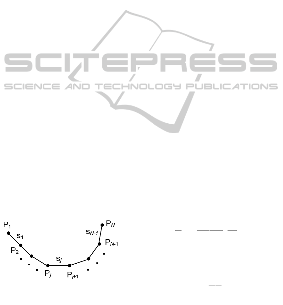
As shown in Figure 1, we assume that a planned
trajectory has N waypoints, P
1
… P
N
, and N-1
segments, s
1
,…,s
N-1
. Each given waypoint P
i
is
described with a 1×6 configuration vector w
i
=[x
i
, y
i
,
z
i
,
ϕ
i
,
θ
i
, ψ
i
]
T
. By using an inverse kinematics
solution, each configuration vector can be converted
into a corresponding joint variables vector q
i
=[q
1i
,
…, q
ni
]
T
.
Before looking for an optimal trajectory planning
solution, one should determine a desired optimality
goal to be achieved, a control method, actual
physical constraints and allowed tolerances of key
trajectory values such as path deviations, constraints
excesses etc.
Figure 1: Trajectory waypoints and segments.
In a particular case of planning continuous jerk
robot trajectories, terminal (initial and final)
positions, velocities and accelerations are known
(they are often equal to zero). Also, velocity and
acceleration constraints for each robot joint are
known (jerk constraints can also be known, but
herein they are not taken into consideration). Quality
assessment criteria include observation of a total
traverse time of a robot along a given path and of a
total execution time of the algorithm needed to
finish trajectory calculations. In the same time,
deficiency assessment criteria include constraints
violations, failures in maintenance of a continuous
jerk in the waypoints, and the inability of a robot
tool to pass through all given waypoints.
Two different trajectory planning methods have
been considered for comparison - a modified
Yakimenko method adapted for robot applications,
and a Ho-Cook “555” method.
2.1 Modified Yakimenko Trajectory
Planning Algorithm
The essence of the Yakimenko method is separation
of the trajectory profile and the actual velocity
profile through selection of a suitable optimization
variable
τ
(t) and its first derivative λ(t)=d
τ
(t)/dt. The
variable
τ
(t) is called a virtual arc, and its derivative
λ(t) is called a velocity factor.
For example, such separation allows us to take
time-varying dynamics of robotic mechanisms into
account during descent along a planned trajectory. In
other words, each trajectory segment may have a
different velocity profile dictated by
τ
(t) and λ(t).
Following this approach, trajectory Γ passing
through a set of given waypoints P
1
,…,P
N
becomes a
function of accompanying configuration vectors
w
1
,…,w
N
, and also a function of a selected
optimization variable
τ
(t), i.e. Γ=w(t)=w(
τ
).
Interpretation of Γ in two different frames allows
also interpretation of a velocity profile in two
separate frames:
() ()
()
(
)
()
()
11
dt
d
t
dt
ddtt
dt
ττ
τ
τλ
′
==
w
ww =w
(1)
If the form of w(
τ
) allows multiple
differentiations with respect to
τ
, then so called
virtual velocities, accelerations, jerks and snaps can
be obtained, as follows:
() () ()
()
() () ()
p
1
1
w
dt d
t
ddt
ttt
t
ττ
τ
λ
λ
−
′
==
==
vw w
wv
(2)
ICINCO 2011 - 8th International Conference on Informatics in Control, Automation and Robotics
482

() () () () ()
2
pp w
tt
τττλ
−
′
′′
===av w a
(3)
() () () () ()
3
pp
τττλ
−
′
′′′
===
w
ttja w j
(4)
() () () () ()
4
p
ττ λ
−
′′′′
′
== =
pw
wt t tsj s
(5)
where v
w
(t), a
w
(t), j
w
(t), and s
w
(t) denote actual
velocities, accelerations, jerks and snaps,
respectively.
When virtual complements are found, one can
use relations (2)-(5) to find v
w
(t), a
w
(t), j
w
(t), and
s
w
(t). In order to get responses of v
w
(t), a
w
(t), j
w
(t),
and s
w
(t) bounded and continuous over all trajectory
segments s
j
, j=1,…,N-1, boundary vectors w
tj
=[w
j
v
wj
a
wj
j
wj
s
wj
]
T
and w
t(j+1)
=[w
j+1
v
w(j+1)
a
w(j+1)
j
w(j+1)
s
w(j+1)
]
T
must be defined for each pair of waypoints
P
j
and P
j+1
, j=1,…,N.
In general, each segment is unique and
accordingly, a number of components of its
boundary vectors can vary.
The travel along segment s
j
starts at t=0 and ends
at t=t
j+1
. A total traverse time is equal to:
1
1
1
N
tot i
i
tt
−
+
=
=
∑
For a given robot tool trajectory planning task,
compound boundary vectors contain only position,
velocity and acceleration components: w
tj
=[w
j
v
wj
a
wj
]
T
, w
t(j+1)
=[w
j+1
v
w(j+1)
a
w(j+1)
]
T
. Having l known
boundary conditions (here l=3+3=6), the minimal
degree of a polynomial that satisfies l conditions is
l+1.
Because of the assumption that initially jerk is
equal to zero and cannot attain any other value than
zero, instead of a seventh-order polynomial, a fifth-
order polynomial can be used to describe segment s
j
:
()
5
0
2345
012345
i
jij
i
j
jj j j j
tt
ttttt
=
∑
w=β
= β +β +β +β +β + β
(6)
Upon differentiation of (6) we obtain:
()
5
1
1
234
12 3 4 5
23 4 5
i
wj ij
i
j
jj j j
tit
tt t t
−
=
⋅
∑
v=β
= β + β + β + β + β
(7)
() ( )
5
2
2
23
23 4 5
1
2 6 12 20
i
wj ij
i
j
jj j
tii t
tt t
−
=
=−
=+ + +
∑
a β
ββ β β
(8)
Letting t in (6) to run from zero to t
j+1
, the
boundary conditions for segment s
j
can be expressed
as:
()
()
111
1
1
1
1
(0) ( )
(0) ( )
(0) ( )
j
jj jj j j
wj wj wj j
wj
wj wj wj j
wj
Pt P
t
t
+++
+
+
+
+
=
===
==
==
ww w w
vv v v
aa a a
(9)
where v
wj
and v
w(j+1)
represent tool velocities, while
a
wj
and a
w(j+1)
represent tool accelerations at points P
j
and P
j+1
, respectively (see Figure 1).
From (6)-(9) we obtain:
()
()
0
1
2
23 4 5
1
11 1 1 13
23 4
1
11 1 14
23
11 15
1
10 0 0 0 0
01 0 0 0 0
00 2 0 0 0
1
012 3 4 5
0 0 2 6 12 20
j
j
wj
j
wj
j
j
jj j j j j
wj
jj j j j
jj jj
wj
tt t t t
tt t t
ttt
+
++ + + +
+
++ + +
++ +
+
⎡⎤
⎡⎤⎡⎤
⎢⎥
⎢⎥⎢⎥
⎢⎥
⎢⎥⎢⎥
⎢⎥
⎢⎥⎢⎥
⎢⎥
⎢⎥⎢⎥
⎢⎥
⎢⎥⎢⎥
⎢⎥
⎢⎥⎢⎥
⎢⎥
⎢⎥⎢⎥
⎢⎥
⎢⎥⎢⎥
⎣⎦⎣⎦
⎣⎦
w
β
v
β
a
β
=
w
β
v
β
β
a
(10)
Initially, only boundary conditions for the first
and last segment are known, as well as all positions
in the given waypoints. The trajectory planning task
is to find unknown velocities and accelerations at the
boundaries of each intermediate segment.
Respecting that
τ
(t) and λ(t) may affect each
trajectory segment s
j
in a different way, we denote
them as
τ
j
and λ
j
.
Let us now define a trajectory segment s
j
as a
function of virtual arc
τ
j
:
()
5
i0
2345
01 2 3 4 5
i
jj ijj
jjjjjjjjjjj
ττ
τ
ττττ
=
++ ++ +
∑
w=b
=b b b b b b
(11)
Upon consecutive differentiations of (11) as in
(2)-(5), and by accounting for boundary vectors
w
tj
=[w
j
v
wj
a
wj
]
T
and w
t(j+1)
=[w
j+1
v
w(j+1)
a
w(j+1)
]
T
, we
obtain the following system of equations:
()
()
0
1
2
23 4 5
1
3
23 4
1
4
23
5
1
10 0 0 0 0
01 0 0 0 0
00 2 0 0 0
1
012 3 4 5
0 0 2 6 12 20
j
j
pj
j
pj
j
j
jf jf jf jf jf j
pj
jf jf jf jf j
jf jf jf j
pj
ττ τ τ τ
ττ τ τ
τττ
+
+
+
⎡⎤
⎡⎤⎡⎤
⎢⎥
⎢⎥⎢⎥
⎢⎥
⎢⎥⎢⎥
⎢⎥
⎢⎥⎢⎥
⎢⎥
=
⎢⎥⎢⎥
⎢⎥
⎢⎥⎢⎥
⎢⎥
⎢⎥⎢⎥
⎢⎥
⎢⎥⎢⎥
⎢⎥
⎢⎥⎢⎥
⎣⎦⎣⎦
⎣⎦
w
b
v
b
a
b
w
b
v
b
b
a
(12)
where
τ
j
f
denotes the virtual crossing length of s
j
.
By solving (12), eventually we obtain:
0
1
2
32 3 2
3
4
43 2 43 2
5
54 35 43
10 0 000
01 0 000
1
00 000
2
10 6 3 10 4 1
22
15831571
2
63 16 31
22
j j
j
j
jf jf jf jf jf jf
j
j
jf jf jf jf jf jf
j
jf jf jf jf jf jf
ττ ττ ττ
ττ τ ττ τ
ττ ττ ττ
⎡⎤
⎢⎥
⎢⎥
⎢⎥
⎡⎤
⎢⎥
⎢⎥
⎢⎥
⎢⎥
⎢⎥
⎢⎥
−−− −
⎢⎥
=
⎢⎥
⎢⎥
⎢⎥
⎢⎥
⎢⎥
−−
⎢⎥
⎢⎥
⎢⎥
⎢⎥
⎣⎦
⎢⎥
⎢⎥
−−− −
⎢⎥
⎣⎦
bw
bv
b
b
b
b
1
(1)
(1)
pj
pj
j
pj
pj
+
+
+
⎡⎤
⎢⎥
⎢⎥
⎢⎥
⎢⎥
⎢⎥
⎢⎥
⎢⎥
⎢⎥
⎣⎦
a
w
v
a
(13)
CONTINUOUS JERK TRAJECTORY PLANNING ALGORITHMS
483

Besides velocities, accelerations and jerks,
coefficients of the fifth-order polynomials to be
found should also provide the continuity of snap
s
w
(t). This is combined with Yakimenko approach to
optimization of velocity profile by minimization of
the traverse time of each trajectory segment. This
should finally result in the shortest total traverse
time t
tot
of the whole trajectory.
The idea is to have simultaneous but separate
changes of λ and
τ
that influence the form of
trajectory defined.
The condition of jerk and snap continuity applied
to two neighboring segments s
j
and s
j+1
results with
the following equalities:
()
()
(
)
()
()
33
11 1
1
00
λτ λ
++ +
+
=→ =
jj j jpjjf j
pj
Tjj j j
(14)
()
()
(
)
()
()
44
11 1
1
00
λτλ
++ +
+
=→ =
jj j jpjjf j
pj
Tss s s
(15)
By combining (12)-(14) and taking also the
position, velocity and acceleration continuity criteria
into account, a jerk continuity relation valid for three
adjacent segments s
j
, s
j+1
and s
j+2
results with the
following equality:
()
() ()
()
()
()
()
33 22
1
1(1)
222
1
22
11212
2
1(1)
22
2
111
333 3
11
1
333
1
8
12
8
3
20 20 20
λλ λλ
λ
τ
τττ
λ λ λλ λλ
λ
ττ τ
τ
λλλ λ
τττ τ
+
++
+
+++++
++
++
+++
++
+
+
⎛⎞
⎜⎟
++ − −
⎜⎟
⎝⎠
⎛⎞
⎜⎟
−+− + =
⎜⎟
⎝⎠
⎛⎞
⎜⎟
=− + + −
⎜⎟
⎝⎠
jj jj
pj pj j p j
jfjf jf
jf
j j jj jj
jpj
pj pj
jf
jf jfjf
jjj j
jj
jf jf
jf j
va v
ava
ww
()
2
3
1
+
+
j
f
w
(16)
that allows calculation of unknown boundary values
in (13):
,,
pj pj
va
(1) (1)
,,
pj pj++
va and
() ()
22
,
pj pj++
va
.
There are
N-2 such segment triples s
j
, s
j+1
and
s
j+2
, and accordingly, N-2 equations of type (16).
Since there are totally 2×(
N-2) unknowns, still N-2
new equations are needed to make the system
solvable. This can be done by introducing a criterion
of snap continuity in each given waypoint, which
results with the following equality:
()
() ()
()
()
()
()
44 33
1
1(1)
32 33
1
22 3 22
11212
2
1(1)
22
22 3 2
111
444
1
444
1f
14 2
16
14 2
3
30 30
λλ λλ
λ
ττ ττ
λ λ λλ λλ
λ
ττ τ τ
λλλ
τττ
+
++
+
+++++
++
++
+++
+
+
+
⎛⎞
⎜⎟
++ − +
⎜⎟
⎝⎠
⎛⎞
⎜⎟
+++ − =
⎜⎟
⎝⎠
⎛⎞
⎜⎟
=− + +
⎜⎟
⎝⎠
jj jj
pj pj j p j
jf jf jf
jf
j j jj jj
jpj
pj pj
jf
jf jf jf
jjj
jj
jf jf
j
va v
ava
ww
()
4
1
12
4
1f
30
λ
τ
+
+
+
+
j
j
j
w
(17)
The equations for boundary segments
s
1
and s
N-1
are different, as initial conditions for
s
1
and final
conditions for
s
N-1
are known. This means that these
values are moved to the right-hand side of equations
(16) and (17), respectively:
1
st
segment – jerk continuity
22
2
12 21
2222
22
2112
223
23 23
1
33 1
23
2
21
33 3 3 3
12 2 1 1
2311
33 3 2
112 2 1
12 3
8
20
8
20 20
λλ λλ
λλ
ττ
ττ
λλ λλ
λ
τττ
λλ λ λ λ
τ
ττ τ τ
⎛⎞⎛⎞
−−+−
⎜⎟⎜⎟
⎜⎟⎜⎟
⎝⎠
⎝⎠
−+=−+
⎛⎞
++ − − −
⎜⎟
⎜⎟
⎝⎠
pp
ffff
pp
f
ff
pp
fff f f
va
va w
wwva
(18)
(
N-1)
th
segment – jerk continuity
()
()
()
33 22
22 21
(2) (2) 1 (1)
222
(2)(2) (2)
1
3
2
12 2
1(1)2
3
(2) (2)
1
33
21
1
33
(2)
1
8
12
320
20 20
λλ λλ
λ
τ
τττ
λλ λ
λ
ττ τ
λλ λ
ττ
−− −−
−−− −
−−−
−
−− −
−−−
−−
−
−− −
−
−
−
⎛⎞
⎜⎟
+
+−−
⎜⎟
⎝⎠
⎛⎞
⎜⎟
−+ =− +
⎜⎟
⎝⎠
⎛⎞
⎜⎟
++ −
⎜⎟
⎝⎠
NN NN
pN pN N pN
NfNf Nf
Nf
NN N
NpNN
Nf Nf
Nf
NN N
N
Nf
Nf
va v
aw
w
() ()
()
333
111
32
111
8
λλ
τ
ττ
−−
−−−
+−
NN
NpNpN
NfNf Nf
wv a
(19)
1
st
segment – snap continuity
33 22
2
12 21
2222
33 2 2
12 21
322 4
23 23
1
331
32 4
22 1
44 4 4 4
12 2 1 1
2311
44 4 3 2
12 2 1 1
16 3
14 2
30
14 2
30 30
λλ λλ
λλ
ττ ττ
λλ λλ
λ
ττ τ
λλ λ λ λ
ττ τ τ τ
⎛⎞⎛⎞
−+−+
⎜⎟⎜⎟
⎜⎟⎜⎟
⎝⎠⎝⎠
+−=−+
⎛⎞
+− + − −
⎜⎟
⎜⎟
⎝⎠
pp
ff ff
pp
ff f
pp
ff f f f
va
va w
wwva
(20)
(
N-1)
th
segment – snap continuity
()
()
()
44 33
22 21
(2) (2) 1 (1)
32 33
(2) (2) (2)
1
22 4
2
12 2
1(1)2
22 4
(2) (2)
1
44
21
44
(2)
1
14 2
16
330
30
λλ λλ
λ
ττ ττ
λλ λ
λ
ττ τ
λλ
ττ
−− −−
−−− −
−− −
−
−− −
−−−
−−
−
−−
−
−
−
⎛⎞
⎜⎟
+
+−+
⎜⎟
⎝⎠
⎛⎞
⎜⎟
+− =− +
⎜⎟
⎝⎠
⎛⎞
⎜⎟
+−
⎜⎟
⎝⎠
NN NN
pN pN N pN
Nf Nf Nf
Nf
NN N
NpNN
Nf Nf
Nf
NN
N
Nf
Nf
va v
aw
w
() () ()
444
111
1
43 2
11 1
14 2
30
λλλ
ττ τ
−−−
−− −
+−+
NNN
NpNpN
Nf Nf Nf
wva
(21)
In order to simplify derived equations and
organize them in a matrix formulation, the following
substitutions have been introduced (
i=1,…,N-2):
Equation (16)
3
0
2
8
λ
τ
=
j
i
v
jf
K
,
3
0
λ
τ
=
j
i
a
j
f
K
,
()
22
1
11
22
1
12
λλ
λ
ττ
+
+
+
⎛⎞
⎜⎟
=−
⎜⎟
⎝⎠
jj
i
vj
jf
j
f
K
,
()
1
2
11
1
3
λ
λ
λ
τ
τ
+
+
+
⎛⎞
⎜⎟
=− +
⎜⎟
⎝⎠
j
j
i
aj
jf
jf
K
,
()
2
12
2
2
1
8
λ
λ
τ
++
+
=−
jj
i
v
j
f
K
,
()
2
12
2
1
λ
λ
τ
+
+
+
=
jj
i
a
jf
K
,
3
0
3
20
λ
τ
=−
j
i
p
j
f
K
,
()
33
1
1
33
1
20
λλ
ττ
+
+
⎛⎞
⎜⎟
=+
⎜⎟
⎝⎠
jj
i
p
jf
jf
K
,
()
3
1
2
3
1
20
λ
τ
+
+
=−
j
i
p
jf
K
.
ICINCO 2011 - 8th International Conference on Informatics in Control, Automation and Robotics
484

Equation (17)
4
0
3
14
λ
τ
=
j
i
v
jf
L
,
4
0
2
2
λ
τ
=
j
i
a
j
f
L
,
()
33
1
11
33
1
16
λλ
λ
ττ
+
+
+
⎛⎞
⎜⎟
=−
⎜⎟
⎝⎠
jj
i
vj
jf
j
f
L
,
()
22
1
2
11
22
1
3
λ
λ
λ
τ
τ
+
+
+
⎛⎞
⎜⎟
=−
⎜⎟
⎝⎠
jj
i
aj
jf
jf
L
,
()
3
12
2
3
1
14
λ
λ
τ
++
+
=
jj
i
v
j
f
L
,
()
22
12
2
2
1
2
λ
λ
τ
++
+
=−
jj
i
a
j
f
L
,
4
0
4
30
λ
τ
=−
j
i
p
j
f
L
,
()
44
1
1
44
1
30
λλ
ττ
+
+
⎛⎞
⎜⎟
=−
⎜⎟
⎝⎠
jj
i
p
jf
jf
L
,
()
4
1
2
4
1
30
λ
τ
+
+
=
j
i
p
jf
L
.
Equation (18)
3
1
1
0
2
1
8
λ
τ
=−
v
f
K ,
3
1
1
0
1
λ
τ
=−
a
f
K
Equation (19)
()
3
2
1
2
1
8
λ
τ
−
−
−
=
N
N
Fv
Nf
K ,
()
3
2
1
1
λ
τ
−
−
−
=−
N
N
Fa
Nf
K
Equation (20)
4
1
1
0
3
1
14
λ
τ
=−
v
f
L ,
4
1
1
0
2
1
2
λ
τ
=−
a
f
L
Equation (21)
()
4
2
1
3
1
14
λ
τ
−
−
−
=−
N
N
Fv
Nf
L ,
()
4
2
1
2
1
2
λ
τ
−
−
−
=
N
N
Fa
Nf
L .
Using these substitutions, let us define a vector
with elements equal to known components at the
right-hand sides of equations (16)-(21):
()
()
()
()
11111
1
1223010 10 1
222
2
021324
333
-3
031221
222
-2
0211
1
2
-3
-2
−−−
−−−
−−−
−−
⎡⎤
++−−
⎢⎥
⎢⎥
++
⎢⎥
⎢⎥
⎢⎥
⎢⎥
⎢⎥
⎢⎥
++
⎢⎥
++
⎢⎥
==
⎢⎥
⎢⎥
⎢⎥
⎢⎥
⎢⎥
⎢⎥
⎢⎥
⎢⎥
⎢⎥
⎢⎥
⎢⎥
⎣⎦
j
pppvpap
j
ppp
NNN
jN
pN pN pN
NNN
jN
pN pN F p
p
s
s
sN
sN
KKKKK
KKK
KKK
KKK
h
wwwv a
h
www
h
www
h
ww
h
h
h
h
h
22
11111
1223010 10 1
222
021324
333
031221
22222
0211
−−
−−−
−−−
−−−−−
−−
⎡⎤
⎢⎥
⎢⎥
⎢⎥
⎢⎥
⎢⎥
⎢⎥
⎢⎥
⎢⎥
⎢⎥
−−
⎢⎥
⎢⎥
++−−
⎢⎥
++
⎢⎥
⎢⎥
⎢⎥
⎢
⎢
⎢
++⎢
⎢
++−−
⎣⎦
NN
NFvpNFapN
pppvpap
ppp
NNN
pN pN pN
NNNNN
pN pN FpNFvpNFapN
KK
LLLLL
LLL
LLL
LLLLL
wv a
wwwv a
www
www
wwwva
⎥
⎥
⎥
⎥
⎥
(22)
The equations attain a final matrix form:
11 11
1122
222222
2
00 11 22
3
1
00
2
1
11 11
1122
222222
0011 22
3
0
00
2
1
00
0
00
00 0
0
0
00
0
00
00
0
−
−
⋅==
⎡⎤
⎢⎥
⎢⎥
⎢⎥
⎢⎥
⎢⎥
⎢⎥
⎢⎥
⎢⎥
⎢⎥
⎢⎥
⎢⎥
⎢⎥
⎢⎥
⎢⎥
⎢⎥
⎢⎥
⎢⎥
⎣⎦
pp p
va va
p
vavava
p
v
ii
va
N
a
vava
vavava
v
ii
va
N
a
KKKK
KKKKKK
K
KK
K
LLLL
LLLLLL
L
LL
L
Md h
v
a
()
2
3
3
4
1−
⎡⎤
⎢⎥
⎢⎥
⎢⎥
⎢⎥
⎢⎥
⎢⎥
⎢⎥
=
⎢⎥
⎢⎥
⎢⎥
⎢⎥
⎢⎥
⎢⎥
⎢⎥
⎣⎦
p
p
p
p
pj
pj
pN
v
a
v
h
v
a
a
(23)
The dimensions of matrix M
p
are (2N-4)×(2N-4).
The elements of M
p
are functions of “virtual times”
defined by the optimized values of
τ
and λ, vector d
p
contains values of velocities and accelerations that
must be found, and vector h
p
contains known initial
values defined in (22). Vector d
p
can be calculated
from (23):
1−
=
⋅
p
pp
dMh
(24)
Solving (24) for d
p
starts with calculation of h
p
and M
p
. In order to find the elements of M
p
, initial
values of
τ
j
and λ
j
must be chosen before starting an
iterative process of trajectory optimization. The
initial value of
λ is very important, as it influences a
final result. For the sake of computational simplicity,
the assumption is made that all trajectory segments
start with the same initial value of
λ. For example, in
the trajectory planning example that follows, the
initial value of
λ has been set to 1.5. Because
dynamics of robotic systems change during motion,
any attempt to plan trajectories with inapt initial
values of
λ can end up with noticeable excesses of
velocity, acceleration and jerk constraints.
Therefore, the use of velocity and acceleration
constraints leads iteratively to two new values of
λ.
In the i
th
iteration of the algorithm, new values of λ
are calculated using a Schur-Hadamard quotient:
[
]
()
1
1
max
i
k
i
−
−
=
⎡
⎤
⎣
⎦
I
λ
λ
(25)
where λ is (
N-1)×1 vector and k denotes a number of
a robot joint,
k=1,…, n.
The initial value of
τ
depends on the variable
being optimized along the trajectory. Regardless
from the fact that
τ
can be an arbitrary variable, the
algorithm needs some initial value of
τ
. In the
trajectory planning experiment that follows, this
value has been set to one. Based on the initial
settings of
τ
j
and λ
j
, h
p
and M
p
can be calculated.
Then, using equation (13) the coefficients of the
fifth-order polynomial (11), and consequently, the
expressions for v
pj
and a
pj
can be obtained. Then, by
knowing
λ and using (2) and (3), the polynomials of
the velocity vector v
w
(t) and the acceleration vector
a
w
(t) can be found. The next task is comparison of
the maximal values of v
w
(t) and a
w
(t) and the
respective constraints. If their differences exceed a
given threshold, then a new value of
τ
j
must be
determined. This is done in the following way:
CONTINUOUS JERK TRAJECTORY PLANNING ALGORITHMS
485

() () () ()
110 11
220 22
0
110 11
1
,
,
1max
,
,
fva
fva
jf j vj aj
Nf N vN aN
i
i
ττ εε
ττ εε
ττ εε
ττ εε
−− −−
−
⎡⎤
⎡⎤⎡⎤ ⎡ ⎤
⎢⎥
⎢⎥⎢⎥ ⎢ ⎥
⎢⎥
⎢⎥⎢⎥ ⎢ ⎥
⎢⎥
⎢⎥⎢⎥ ⎢ ⎥
⎢⎥
=+
⎢⎥⎢⎥ ⎢ ⎥
⎢⎥
⎢⎥⎢⎥ ⎢ ⎥
⎢⎥
⎢⎥⎢⎥ ⎢ ⎥
⎢⎥
⎢⎥⎢⎥ ⎢ ⎥
⎢⎥
⎢⎥⎢⎥ ⎢ ⎥
⎣⎦⎣⎦ ⎣ ⎦
⎣⎦
(26)
where operator
denotes a Schur-Hadamard inner
product operation (component wise multiplication),
τ
j0
is the initial value of
τ
j
, and ε
vj
and ε
aj
are relative
velocity and acceleration deviations expressed in
joint space for each joint (
k=1,…n) by:
()
max
max
max
max 1
jk
vj k
k
q
q
⎡⎤
⎛⎞
⎢⎥
⎜⎟
=−
⎢⎥
⎜⎟
⎢⎥
⎝⎠
⎣⎦
ε
(
)
max
max
max
max 1
jk
aj k
k
q
q
⎡⎤
⎛⎞
⎛⎞
⎢⎥
⎜⎟
⎜⎟
=−
⎢⎥
⎜⎟
⎜⎟
⎜⎟
⎢⎥
⎝⎠
⎝⎠
⎣⎦
ε
(27)
Iteratively obtained variables
τ
and λ define
different traverse times for different joints, and this
must be finally reduced to a common time interval,
which would ensure that excesses of imposed
velocity and acceleration limits are avoided. One
simple solution would be to take the largest traverse
time as a common time for all joints. Unfortunately,
this will not prevent possible excesses of limits
because not only absolute values, but also the
relations among traverse times play an important
role.
The other way to solve the problem is extension
of all traverse times by introducing an auxiliary
scaling factor that intentionally decreases the values
of given limits. The idea is not to find the shortest
time intervals but to obtain the best average total
traverse time that keeps joint velocities and
accelerations within limits. Finally, the resultant
interval is picked by applying the max-operator to
all intervals. That approach usually results with
slightly longer traverse times, but nevertheless, it is
very useful in the systems with time-varying
dynamics such as those in robotics. It should be
noted that the use of the auxiliary scaling factor is
not necessary for off-line planning.
2.2 Ho-Cook ”555” Trajectory
Planning Algorithm
In order to compare a modified Yakimenko method
with some method of its kind, a Ho-Cook “445”
method described in [8] has been changed to a “555”
method, indicating that all trajectory segments from
s
1
to s
N-1
are described with fifth-order polynomials
defined in equation (6). This means that the
coefficients of the polynomials should provide the
continuity of v
w
(t), a
w
(t), j
w
(t), and s
w
(t). The “555”
method calculates coefficients of fifth-order
polynomials starting from equation (10), which
means that the solution is searched directly in the
time domain. Under the continuity of jerk and snap
condition for
τ
=λ=1, equation (16) assumes the
following form:
112
222 2
1
11
212
333 3
1
11 11 11 1
812 3 8
11111
20 20 20
jj j j j
jjj
jjj j
jj jj
j
jjj j
tttttt t
ttttt
+
++
+
++
+++
+
⎛⎞⎛⎞
++ − − + −
⎜⎟⎜⎟
⎜⎟
⎜⎟
⎝⎠⎝⎠
⎛⎞
+=−++ −
⎜⎟
⎜⎟
⎝⎠
va v a v
aw ww
(28)
Thus, equation (17) attains a simpler form:
112
32 33 22 3
11 1
212
24444
111
11 11 11 1
14 2 16 3 14
1111 1
23030 30
jj j j j
jj jj jj j
jj jj
jjjjj
tt tt tt t
ttttt
+
++
++ +
+++
+++
⎛⎞⎛⎞
++− +− +
⎜⎟⎜⎟
⎜⎟⎜⎟
⎝⎠⎝⎠
⎛⎞
−=−+−+
⎜⎟
⎜⎟
⎝⎠
va v a v
aw ww
(29)
The rest of the algorithm resembles the steps of
the modified Yakimenko method and ends up with
the matrix equation similar to equation (24):
1
s
ss
−
=dMh
(30)
The Ho-Cook “445” method calculates travel
times for each segment based on the normalized
distance between
P
j
and P
j+1
expressed in joint
coordinates and iteratively corrected by the ratio
factor between the maximal velocities and
accelerations on one hand, and the given velocity
and acceleration constraints on the other.
In contrast to the “445” method, “555” method
calculates relative velocity and acceleration
deviations expressed by (27) and thereafter it adjusts
iteratively the travel times of each trajectory
segment
s
i
:
() () ()
10 1 1
1
20 2 2
2
10 1 1
1
11
1
abs 1 abs 1
2
va
va
vj aj
j
NvNaN
N
i
ii
t
t
t
t
t
t
t
εε
εε
εε
εε
−−−
−
−−
⎛
⎛⎞⎛⎞
⎡⎤ ⎡ ⎤ ⎡ ⎤
⎡⎤
⎜⎟⎜⎟
⎢⎥ ⎢ ⎥ ⎢ ⎥
⎢⎥
⎜⎟⎜⎟
⎢⎥ ⎢ ⎥ ⎢ ⎥
⎢⎥
⎜⎟⎜⎟
⎢⎥ ⎢ ⎥ ⎢ ⎥
⎢⎥
⎜⎟⎜⎟
=+++
⎢⎥ ⎢ ⎥ ⎢ ⎥
⎢⎥
⎜⎟⎜⎟
⎢⎥ ⎢ ⎥ ⎢ ⎥
⎢⎥
⎜⎟⎜⎟
⎢⎥ ⎢ ⎥ ⎢ ⎥
⎢⎥
⎜⎟⎜⎟
⎢⎥ ⎢ ⎥ ⎢ ⎥
⎢⎥
⎜⎟⎜⎟
⎢⎥ ⎢ ⎥ ⎢ ⎥
⎢⎥
⎣⎦
⎣⎦ ⎣ ⎦ ⎣ ⎦
⎝⎠⎝⎠
⎞
⎜⎟
⎜⎟
⎜⎟
⎜⎟
⎜⎟
⎜⎟
⎜⎟
⎜⎟
⎝⎠
(31)
The enhancement of this procedure can be
obtained by additional correction of a segment travel
time having the following form:
,1,2
ic c s i
ki
=
⋅=t η t
(32)
ICINCO 2011 - 8th International Conference on Informatics in Control, Automation and Robotics
486
where k
c
is an auxiliary correction factor, and
s
η
is
determined by the relative magnitude of velocity and
acceleration with respect to the given constraints:
(
)
max min
max ,
jj
sv
smx
⎡⎤
⎢⎥
=
⎢⎥
⎣⎦
vv
η
v
()
max min
1
2
max ,
jj
sa
smx
⎡⎤
⎢⎥
=
⎢⎥
⎣⎦
aa
η
a
(
)
max ,
ssvsa
=ηηη
(33)
Once the polynomials have been defined for all
robot joints, the result obtained in this way can
undergo further optimization (using GA, for
example), which is the subject of ongoing research
work.
3 SIMULATION RESULTS
Let us apply two trajectory planning methods to a 3
DOF robot shown in Figure 2. The lengths of robot
segments are
d
1
= 1.1 m, and d
2
= 0.9 m. Using the
following equations for forward kinematics, the path
and orientation of the robot tool are determined:
() ( )
() ( )
11212
11212
123
cos cos
sin sin
j
jjj
jj jj
jjjj
X
dFd FF
Yd F d F F
OFF F
=++
=++
=++
(34)
where
X
j
and Y
j
represent x- and y-coordinate of P
j
,
and
O
j
represents the orientation of robot tool at P
j
.
Twelve given robot tool waypoints, starting with
P
1
=(1.0, 0.5, 0), form a triangle with vertices (1, 0,
0), (0, 1, 0) and (1, 1, 0). Velocity and acceleration
vectors at both ends of the trajectory are set to v
1
T
=
v
N
T
= [-0.1, 0.4, 0] rad/s, a
1
T
= a
12
T
= [1, 3, 0] rad/s
2
.
Being convenient, maximal velocities and
accelerations of all joints are set to 2 rad/s and 10
rad/s
2
, respectively.
Initial values of Yakimenko parameters are:
τ
j0
=1, λ
0
=1.5.
d
1
d
2
x
Ft
1
()
Ft
2
()
Ft
3
()
y
Figure 2: A three degree of freedom planar robot.
The given waypoints are found in the robot joint
space using the robot inverse kinematics equations:
()
()
()
()
()
()
2222
12
2
12
12 2 2 2
1
12 2 2 2
312
arccos
2
cos sin
arctan
cos sin
⎛⎞
+−−
=
⎜⎟
⎜⎟
⎝⎠
⎛⎞
+⋅−⋅
⎜⎟
=
⎜⎟
+
⋅+ ⋅
⎝⎠
=−−
jj
j
jj jj
j
jj jj
jjjj
XYdd
P
dd
dd P Yd P X
P
dd P X d P Y
POPP
(35)
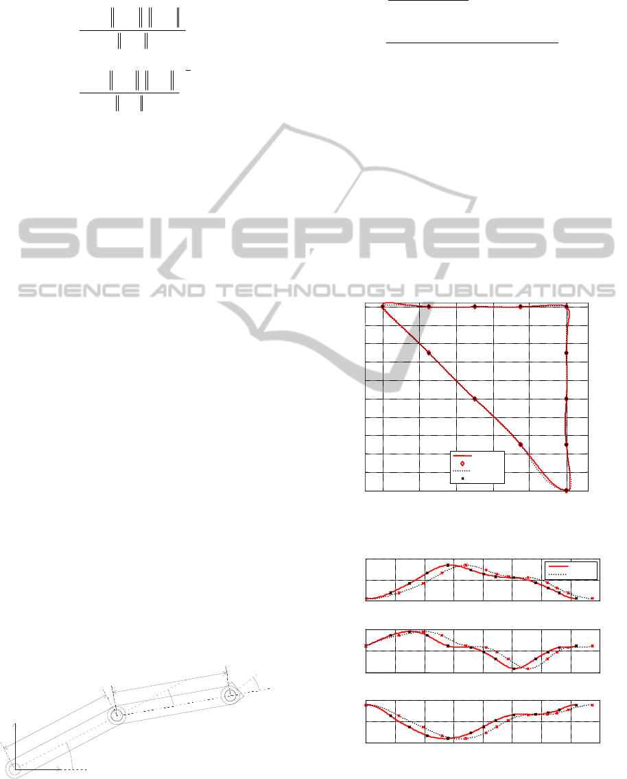
The analysis of trajectory planning results shows
that the planned trajectories have a similar shape
since both pass through the same waypoints (Figure
3). Path deviations obtained with the Ho-Cook
“555” algorithm are similar to those obtained with
the adapted Yakimenko method. Achievement of
higher accuracy requires addition of new waypoints,
for example, by using a well known Taylor bounded
deviations method (Taylor, 1979). It can also be
noticed in Figure 4 that the traverse time of the
“555” trajectory is comparable to the time of the
“Yakimenko” trajectory (3.9 s compared to 3.6 s).
0 0.2 0.4 0.6
0.8
1
0
0.1
0.2
0.3
0.4
0.5
0.6
0.7
0.8
0.9
1
x
y
Yakimenko vs. „555“ method
Yakimenko
Waypoints
„555“
Waypoints
Figure 3: Planned trajectories.
0 0.5 1 1.5 2
2.5
3
3.5 4
-1
0
1
t
(s)
Yakimenko vs. „555“ method
Yakimenko
„555“
0 0.5 1 1.5 2
2.5
3
3.5 4
1.5
2
2.5
t
(s)
0 0.5 1 1.5 2
2.5
3
3.5 4
-3
-2
-1
t
(s)
q
1
(rad)
(rad)
(rad)
q
2
q
3
Figure 4: The position of robot joints.
CONTINUOUS JERK TRAJECTORY PLANNING ALGORITHMS
487
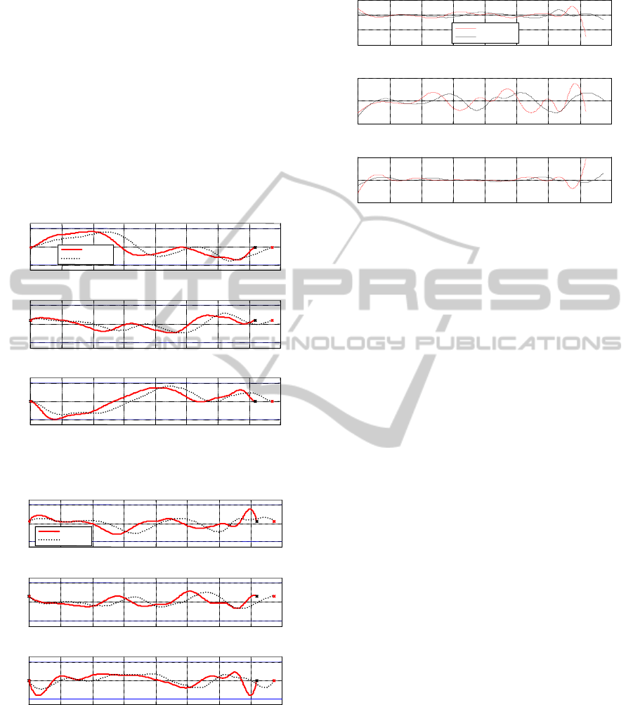
All velocities (Figure 5) and accelerations
(Figure 6) of robot joints obtained with considered
algorithms are smooth and they all stay within the
given constraints. Also, all velocities and
accelerations are equal to the requested velocity and
acceleration values at the start and the end of the
trajectories.
Analyzing the jerk responses shown in Figure 7,
one can see that all interpolation methods ensure the
continuity of jerk, but the responses obtained with
the “555” method are smoother. General conclusions
cannot be made as the result of the Yakimenko
method depends on
τ
j0
and λ
0
.
0
0.5
1
1.5
2
2.5
3
3.5 4
-2
0
2
t
(s)
d
q
1
/d
t
(rad/s)
Yakimenko vs. „555“ method
Yakimenko
555
0
0.5
1
1.5
2
2.5
3
3.5 4
-2
0
2
t
(s)
(rad/s)
0
0.5
1
1.5
2
2.5
3
3.5 4
-2
0
2
t
(s)
(rad/s)
d
q
2
/dt
dq
3
/dt
Figure 5: The velocity of robot joints.
0
0.5
1
1.5
2
2.5
3
3.5 4
-10
0
10
t
(s)
(rad/s
2
)
Yakimenko vs. „555“ method
Yakimenko
555
0
0.5
1
1.5
2
2.5
3
3.5 4
-10
0
10
t
(s)
0
0.5
1
1.5
2
2.5
3
3.5 4
-10
0
10
t
(s)
(rad/s
2
)
(rad/s
2
)
d
2
q
1
/dt
2
d
2
q
2
/dt
2
d
2
q
3
/dt
2
Figure 6: The acceleration of robot joints.
0 0.5 1 1.5 2
2.5
3
3.5 4
-200
-100
0
100
Yakimenko VS. „555“ method
t
(s)
(
rad/s
3
)
Yakimenko
„555“
0 0.5 1 1.5 2
2.5
3
3.5 4
-50
0
50
t
(s)
0 0.5 1 1.5 2
2.5
3
3.5 4
-200
0
200
t
(s)
(
rad/s
3
)
(
rad/s
3
)
d
3
q
1
/
dt
3
d
3
q
2
/
dt
3
d
3
q
3
/
dt
3
Figure 7: The jerk of robot joints.
4 CONCLUSIONS
There are many robot applications which require
smooth robot motion. Both iterative trajectory
planning algorithms described in this paper ensure
the continuity of velocity, acceleration, and jerk at
all trajectory segments. Moreover, the velocities and
accelerations at the terminal points can assume
different values. The first method, called a modified
Yakimenko method achieves jerk continuity by
splitting a trajectory into a planned path and a
corresponding velocity profile defined by a selected
optimization criterion (or more of them), while the
other method, called a Ho-Cook “555” method uses
fifth-order polynomials to achieve the same goal in
the time domain.
The Ho-Cook “555” method shows more
potential when the shortest traverse times are
important. On the other hand, the modified
Yakimenko method is much more apt when other
optimizations (shortest path, minimal energy
consumption, minimal path deviation etc.) are also
considered. In the paper it has been shown that both
methods give similar results of trajectory planning if
the optimization criterion was to get close to the
given velocity and acceleration limits.
Regarding a future work, both methods will be
further investigated in terms of applying various
optimization methods (e.g. genetic algorithms) and
combining various optimization criteria. Also, the
future work will be more focused on the extensive
laboratory experiments with the available robotic
systems.
ICINCO 2011 - 8th International Conference on Informatics in Control, Automation and Robotics
488

ACKNOWLEDGEMENTS
The work in this paper was performed within the
project “Integrated Control of Robotic Systems in
Complex Environments” that was supported by a
grant from the Croatian Ministry of Science,
Education and Sports.
REFERENCES
Biagiotti, L., Melchiorri, C., 2008. Trajectory Planning for
Automatic Machines and Robots, Springer-Verlag
Berlin Heidelberg.
Kyriakopoulos, K. J., Saridis, G. N., 1988. Minimum jerk
path generation, In Proceedings of the IEEE
International Conference on Robotics and
Automation, 364–369.
Macfarlane, S., Croft, E. A., 2003. Jerk-Bounded
Manipulator Trajectory Planning: Design for Real-
Time Applications, In IEEE Transactions on Robotics
and Automation, Vol.19, No. 1, 42-52.
Li, H., Ceglarek, D., 2002. Optimal Trajectory Planning
for Material Handling of Compliant Sheet Metal Parts,
In ASME Journal of Mechanical Design, Vol. 124,
213-222.
Ho, C. Y., Cook, C.C., 1982. The application of spline
functions to trajectory generation for computer
controlled manipulators, In Digital Systems for
Industrial Automation, 1 (4): 325-333.
Ranky, P.G., Ho, C.Y., 1985. Robot Modelling – Control
and Applications with Software, Springer-Verlag, IFS
(Publications) Ltd, UK.
Kovacic, Z., Bogdan, S., Petrinec, K., Reichenbach, T.,
Puncec, M., 2001. Leonardo - The Off-line
Programming Tool for Robotized Plants, In CD-ROM
Proceedings of the 9th Mediterranean Conference on
Control and Automation, Dubrovnik, Croatia.
Petrinec, K., Kovacic, Z., 2005. The application of spline
functions and Bézier curves to AGV path planning, In
CD-ROM Proceedings of the IEEE International
Symposium on Industrial Electronics ISIE 2005,
Dubrovnik, Croatia.
Petrinec, K., Kovacic, Z., 2007. Trajectory planning
algorithm based on the continuity of jerk, In
Proceedings of the 15th Mediterranean Conference on
Control and Automation, Athens, Greece, T30-041.
Yakimenko, O. A., 2006. Direct Method for Real-Time
Prototyping of Optimal Control, In Proceedings of the
International Control Conference, Glasgow, Scotland.
Bevilacqua, R., Yakimenko, O., Romano, M., 2006. On-
Line Generation of Quasi-Optimal Docking
Trajectories, In Proceedings of the 7th International
Conference on Dynamics and Control of Systems and
Structures in Space (DCSSS), Greenwich, London,
England.
Kaminer, I., Yakimenko, O., Pascoal, A., Ghabcheloo, R.,
2006. Path Generation, Path Following and
Coordinated Control for Time-Critical Missions of
Multiple UAVs, In American Control Conference,
4906–4913.
Taylor, R. H., 1979. Planning and execution of straight
line manipulator trajectories, In IBM J. Research and
Development, Vol. 23, 424-436.
CONTINUOUS JERK TRAJECTORY PLANNING ALGORITHMS
489
