EXPERIMENTAL RESULTS OF INTEGRAL SLIDING MODE

CONTROLLER FOR A NONHOLONOMIC MOBILE ROBOT

Alaa Dib and Houria Siguerdidjane

SUPELEC, Systems Sciences (E3S), 91192, Gif-sur-Yvette cedex, France

Keywords:

Mobile Robot, Trajectory Tracking, Integral Sliding Mode, Nonholonomic systems.

Abstract:

This paper addresses the trajectory tracking problem of a nonholonomic mobile robot. More precisely, we are

interested in solving the problem of tracking a reference trajectory in presence of disturbances. A control strat-

egy based on the Integral Sliding Mode is proposed combined with a state feedback linearization. While many

studies have considered the kinematic model of the vehicle only, we have used both kinematic and dynamic

models. The distinctive property of the proposed controller is its robustness of performance in the presence

of uncertainties. To assess the quality of the proposed approach, we performed in addition to simulations the

implementation of this controller on the robot Koala, a two-wheel differentially driven mobile robot. Lab work

illustrates the real quality and efﬁciency of this control strategy.

1 INTRODUCTION

The motion control of mechanical systems under non-

holonomic constraints has received much attention

during past years. Wheeled mobile robots and car-

like vehicles are typical examples of such systems. As

pointed out in an early paper of Brockett (Brockett,

1983), such control systems cannot be stabilized by

continuously differentiable, time invariant, state feed-

back control laws. Another difﬁculty in controlling

nonholonomic mobile robots is that in the real world

there are uncertainties in their modeling. Taking into

account intrinsic characteristics of mobile robots such

as actual vehicle dynamics, inertia and power limits of

actuators and localization errors, their dynamic equa-

tions could not be described as a simpliﬁed mathemat-

ical model. This has attracted interest of researchers

to the problem of nonholonomic mobile robot con-

trol. Discontinuous state feedback controller is used

(Astolﬁ, 1995), (Astolﬁ, 1996)), tracking control us-

ing direct Lyapunov method (D’Andrea-Novel et al.,

1995), time variant state feedback (Samson, 1995),

(Walsh et al., 1994). Stabilization and control of non-

holonomic systems with dynamic equations are pre-

sented in (Bloch et al., 1992), backstepping based

methods has been considered in several papers (Fierro

and Lewis, 1997), (Jiang and Nijmeijer, 1997), (Tan-

ner and Kyriakopoulos, 2002) and a switched ﬁnite-

time control algorithm has been proposed in (Banavar

and Sankaranarayanan, 2006).

Sliding mode control has been applied to the tra-

jectory control of robot manipulators (Slotine and

Sastry, 1983), (Yeung and Chen, 1988), and is receiv-

ing increasing attention from researches on control

of nonholonomic systems with uncertainties. For ex-

ample, in (Guldner and Utkin, 1994) a sliding mode

control was used to guarantee exact tracking of tra-

jectories made by navigation functions. In (Yang and

Kim, 1999) a sliding mode control law is proposed for

asymptotically stabilizing the mobile robot to a de-

sired trajectory, where robot posture was represented

using polar coordinates. The beneﬁts of the sliding

mode command which makes it very important is its

robustness with regards to disturbances and structural

uncertainties, i. e. the system response depends on the

gradient of the sliding surface and remains insensitive

to variations of system parameters and external distur-

bances. However, during the reaching phase (before

Sliding Mode occurs), the system has no such insen-

sitivity property; therefore, insensitivity cannot be en-

sured throughout an entire response. The robustness

during the reaching phase is normally improved by

high-gain feedback control. Stability problems that

arise inevitably limit the application of such high-gain

feedback control schemes.

In this paper, we propose to perform a feedback

linearization for a class of nonholonomic dynamic

systems, combined with an Integral Sliding Mode

controller which concentrates on the robustness of the

motion in the whole state space. The order of the mo-

tion equation in this type of Sliding Mode is equal

to the dimension of the state space. Therefore, the

robustness of the system can be guaranteed through-

out an entire response of the system starting from the

445

Dib A. and Siguerdidjane H..

EXPERIMENTAL RESULTS OF INTEGRAL SLIDING MODE CONTROLLER FOR A NONHOLONOMIC MOBILE ROBOT.

DOI: 10.5220/0003648904450450

In Proceedings of the 8th International Conference on Informatics in Control, Automation and Robotics (MORAS-2011), pages 445-450

ISBN: 978-989-8425-75-1

 2011 SCITEPRESS (Science and Technology Publications, Lda.)

initial time instance (Utkin and Shi, 1996). To as-

sess the efﬁciency of this approach, the performance

of the proposed controller has been compared to a tra-

ditional PID controller.

This paper is organized as follows. In Section

2, the general dynamic model of nonholonomic sys-

tems is presented. Feedback linearization is discussed

in Section 3. In Section 4 the main result of Inte-

gral Sliding Mode is introduced, and its application to

solve the tracking problem is discussed in Section 5.

Finally in Section 6, experimental results using Koala

mobile robot are discussed, before presenting the con-

cluding remarks in Section 7.

2 MODELLING

The dynamical model of a nonholonomic system is

expressed as (see (Campion et al., 1991b) for details)

M(q)

q+ f(q,

q) = B(q)τ+ A(q)λ

(q)

q = 0

(1)

where q ∈ R

is an n-vector of generalized conﬁgu-

ration variables, M(q) ∈ R

n×n

is a positive deﬁnite

symetric inertia matrix, f(q,

q) ∈ R

denotes the fric-

tion vector, A

(q) ∈ R

m×n

is the matrix associated

with nonholonmic constraints, λ ∈ R

m×1

is a vector

of Lagrange multipliers and B(q)τ ∈ R

is the set of

generalized forces applied to the system. As shown

in (Campion et al., 1991b) it can be written in state

space form as

q = G(q)v

J(q)

v+ m(q, v) = G

(q)B(q)τ

(2)

where v ∈ R

is the vector of pseudo-velocities and

we have

q = G(q)v, where G(q) is a matrix whose

columns are a basis for the null space of A

(q), so

that A

(q)G(q) = 0 and we have

J(q) = G

(q)M(q)G(q)

m(q, v) = G

(q)M(q)

G(q) + G

(q)f(q,

(3)

Under the assumption that det(G

(q)B(q)) 6= 0, it

is possible to perform a partial linearization via feed-

back on (2) by letting

τ =



(q)B(q)



−1

(J(q)u+ m(q, v)) (4)

where u ∈ R

is the pesudo-acceleration vector. The

resulting system is then

q = G(q)v

v = u

(5)

By deﬁning the state q

= (q, v), system (5) can

be expressed as



G(q







u (6)

which is known as the second-order kinematic model

of the constrained mechanical system.

The following two properties of the system (6)

have been established in (Campion et al., 1991a)

• The nonholonomic system (6) is controllable.

• The equilibrium point x

∗

= 0 of the nonholonomic

system (6) can be made Lagrange stable, but can

not be made asymptotically stable by a smooth

state feedback.

3 REVIEW OF FEEDBACK

LINEARIZATION

For the reader convenience, let’s review feedback lin-

earization as shown in (Campion et al., 1991b). For a

nonholonomic system with n degrees of freedom and

n− m actuators, there exists an output vector function

y = h(q) and a static state feedback control u(q, v)

such that the closed loop is stable, and the output

y = h(q) asymptotically converges to zero. This can

be achieved by feedback linearization.

We start by choosing the output function

y =







n−m







(7)

which depends on the conﬁguration state variable q

only, but not on the state v, such that the largest lin-

earizable subsystem is obtained by differentiating this

output function as follows

y = ▽

h(q)

= ▽

h(q)G(q)v

(8)

By differentiating again, one may write

y = F(q, v) + D(q)u (9)

where

F(q, v) =

∂

∂q

[▽

h(q)G(q)v]G(q)v (10)

D(q) = ▽

h(q)G(q) (11)

By choosing h(q) in such a way that the matrix

D(q) is nonsingular for all q, then linearization is

achieved by the following feedback control

u = D

−1

(q)(z− F(q, v)) (12)

ICINCO 2011 - 8th International Conference on Informatics in Control, Automation and Robotics

446

where z ∈ R

n−m

is the new external control input.

And the resulting system is

y = z (13)

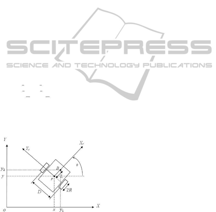
Let’s consider a wheeled mobile robot (WMR)

that is moving on a horizontal plane as shown in Fig.

1. The robot has two independently driven wheels

on a single common axle. The centre of mass of the

robot is located in P(x, y), which is the origin of the

local coordinate frame that is attached to the robot

body and is located on the wheels’ axis. The point

B(x

, y

) is a virtual reference point on x axis of the

local frame at a distance L (lookahead distance) of P.

If the generalized coordinates vector is selected to be

q = [x y θ]

, one velocity constraint is obtained as

xsinθ − ycosθ = 0. Thus, we deﬁne the vector v of

the nonholonomic robot as v = [v ω]

, with v and ω

denote the linear and angular velocities of the robot,

respectively.

The dynamical equations of the mobile can be ex-

pressed in the matrix form (1) where

M(q) =





m 0 0

0 m 0

0 0 I





f(q,

q) = 0

B(q) =





cosθ

sinθ

−





A(q) =





sinθ

−cosθ





λ = −mvω

input-output linearizability is guaranteed through

this choice of output function

y = h(q) = [x+ Lcosθ y + Lsinθ]

(14)

with L 6= 0.

Figure 1: Unicycle mobile robot.

For the sake of completeness, in the next section

we brieﬂy present the major result of Integral Sliding

mode technique presented in (Utkin and Shi, 1996).

4 INTEGRAL SLIDING MODE

For a given dynamic system represented by the fol-

lowing state space equation

˙x = f(x) + B(x)u (15)

where x ∈ R

, u ∈ R

, we suppose that there exists

a feedback control law u = u

(x), such that system

(15) can be stabilized in a desired way (e.g. its state

trajectory follows a reference trajectory with a given

accuracy). We denote this ideal closed loop system as

˙x

∗

= f(x) + B(x)u

(16)

where x

∗

denotes the state trajectory of the ideal sys-

tem under control u

. However, systems like (15)

are normally operating under some uncertainty condi-

tions that may be generated by parameter variations,

unmodeled dynamics and external disturbances etc.

Under this consideration a real control system may be

summarized with

˙x = f(x) + B(x)u+ h

(x, t) (17)

in which function h

(x, t) represents the whole per-

turbation described above and we assume that it is

bounded and fulﬁlls the uncertainty matching condi-

tion, in other words

(x, t) = B(x)u

∈ R

(18)

For system (16), ﬁrstly, we design a control like

u = u

+ u

(19)

where u

is the ideal control deﬁned in (16) and u

designed to be discontinuous for rejecting the pertur-

bation term h

(x, t). Secondly, we design our switch-

ing function s as

s = s

(x) + µ (20)

with s, s

(x), µ ∈ R

This switching function consists of two parts; the

ﬁrst part s

(x) may be designed as the linear combina-

tion of the system states (similar to the conventional

Sliding Mode design); and, the second part µ induces

the integral term and will be determined below.

To derive the Sliding Mode equation, the time

derivative of s on the system trajectories should be

made equal to zero; the differential equation ˙s = 0

should be solved with respect to control input and

the solution u

referred to as the Equivalent Control

should be substituted into the motion equation for u

(Utkin, 1992).

The control philosophy is to design an integral

feedback such that the Equivalent Control is

1eq

= −u

(21)

EXPERIMENTAL RESULTS OF INTEGRAL SLIDING MODE CONTROLLER FOR A NONHOLONOMIC MOBILE

ROBOT

447

Condition (21) holds if

˙µ =

∂s

∂x

( f(x) + B(x)u

)

µ(0) = −s

(x(0))

(22)

where µ(0) is determined based on the require-

ment s(0) = 0 (Sliding Mode occurs starting from the

initial time) . The motion equation of the system in

Sliding Mode will be ideal system (16).

5 TRAJECTORY TRACKING

Given a smooth bounded reference trajectory

(t) = h(q

(t)) (23)

which is generated by a trajectory generator which

satisﬁes nonholonomic constraints, then the track-

ing control problem is to design a feedback control

law for linearized system (13) with output equation

y(t) = h(q(t)) such that the tracking error

e(t) = y(t) − y

(t) (24)

is bounded and asymptotically tends to zero. By dif-

ferentiating (24) twice, one may write using (13)

e =

y−

= z−

+ h

(e, t)

(25)

By applying the algorithm of previous section, we

need to design control z as stated in equation (19):

z = z

+ z

, where z

is predetermined such that sys-

tem x = z

, follows a given trajectory with satisfac-

tory accuracy. For example, z

, may be obtained

through linear feedback control, like z

= −k

x +

, k ∈ R

(n−m)×1

in which gain vector k can be deter-

mined by Pole Placement or Linear Quadratic Regu-

lator (LQR) methods.

We continue by designing the sliding surface

s = c

x+ µ (26)

˙µ = −c

) (27)

µ(0) = −c

x(0) (28)

in that case the motion equation of the Sliding Mode

coincides with that of the ideal system x

= z

, with-

out perturbation. Further more, since s(0) = c

x +

µ(0) = 0, Sliding Mode will occur from the initial

time t = 0. The second part of the control i.e. µ

can be designed as following where m

(x) ≥ |h

The Sliding Mode can be then enforced using the

control

= −M(x)sign(s) (29)

where M(x) is positivedeﬁnite diagonal matrix, under

the condition that matrix

∂s

∂x

B(x) is deﬁnite and the

elements of matrix M(x) are large enough.

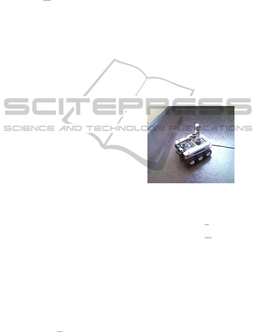
6 EXPERIMENTAL RESULTS

In our experiments, we used the wheeled robot Koala

illustrated in Fig. 2. Koala is a mid-size robot de-

signed for real-world applications. Koala has the

functionality necessary for use in practical applica-

tions, rides on 6 wheels for indoor operations. It

has two-motorized wheels (the middle wheel of each

side), with 0.4 m/s maximum speed, the wheels have

a radius of 4.5 cm and are mounted on an axle 30 cm

long. The chassis of the robot measures 30x30x20

cm (l/w/h) and its total weight is 3.6 kg. Each mo-

tor is equipped with an incremental encoder counting

5850 pulses/turn. The robot is equipped with 16 Infra-

red proximity and ambient light sensors in addition to

a camera mounted on a turret. Data acquisition and

control implementation are performedat sampling pe-

riod T

= 0.05 s.

Figure 2: Mobile robot Koala.

In this section, we will report the experimental re-

sults of Koala in tracking an eight shape reference tra-

jectory deﬁned by

(t) = y

d1max

sin(2π

) + y

d1i

(t) = y

d2max

sin(2π

) + y

d2i

(30)

for t ∈ [0, 2T]. We choose y

d1max

= 2m, y

d2max

= 2m,

d1i

, y

d2i

) = (1.0, 0.0) and T = 40s.

We apply feedback linearization discussed above,

we let q(0) = (0m, 0m, 0rad), i.e., starting with an

initial state error with respect to the assigned trajec-

tory q

(0) = (1.0m, 0.0m, 0.4636rad). In the ﬁrst

set of experiments, PID controller is applied with

= 9.17,k

= 0.72 and k

= 10.59. As we can see

from Figs. 3, a relatively high tracking errors (up to

10.0 cm) are observed on x, y. These tracking errors

are resulting from unmodeled dynamics (motors dy-

namics and unmodeled friction forces) and measure-

ments errors. In addition, there is a large transient

error resulting from the initial posture being different

from the desired trajectory starting point.

ICINCO 2011 - 8th International Conference on Informatics in Control, Automation and Robotics

448

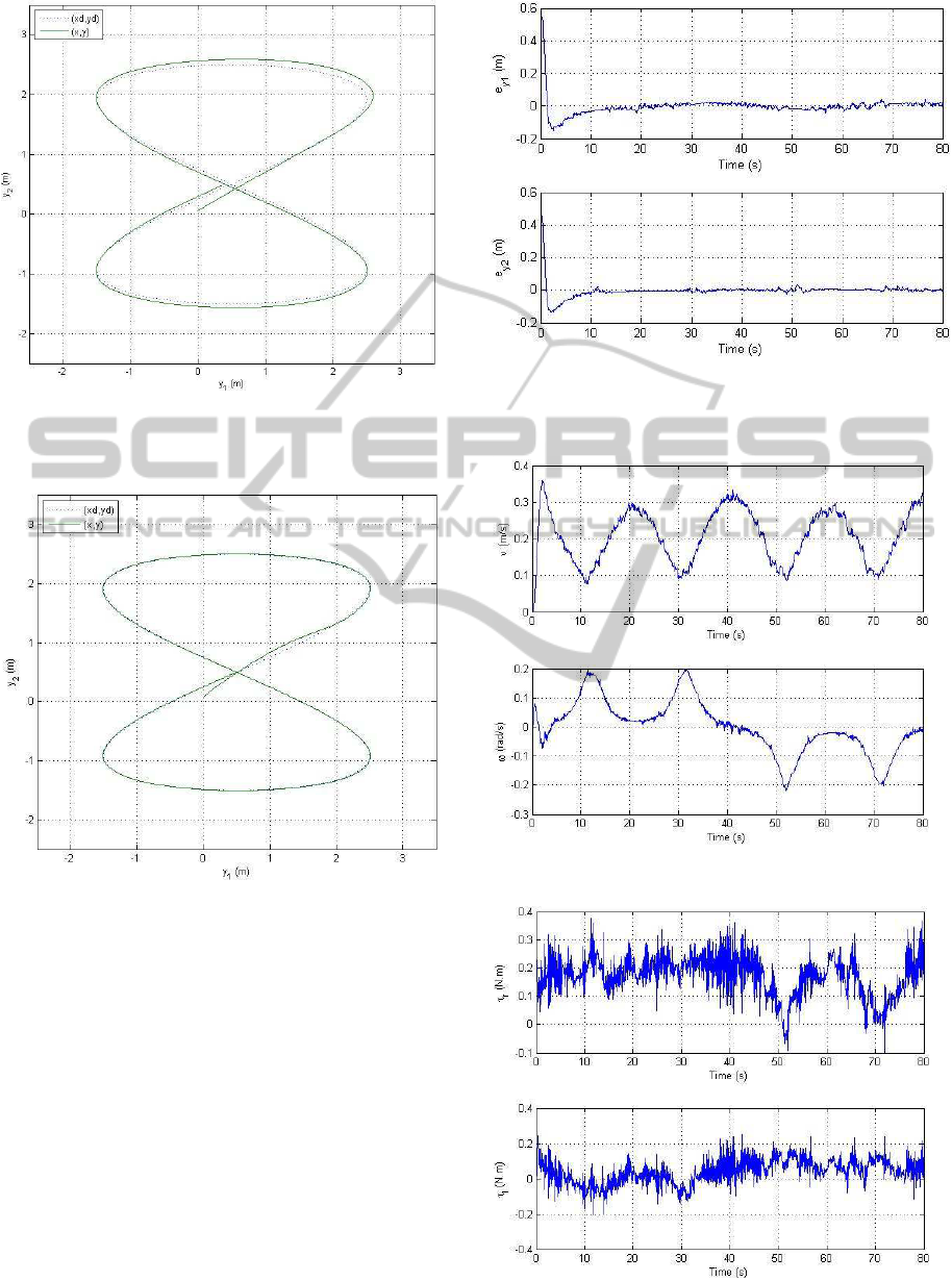
Figure 3: Asymptotic trajectory tracking using linear PID

controller to track an eight shape trajectory on the (x, y)

plane.

Figure 4: Asymptotic trajectory tracking using Integral

Sliding Mode controller of an eight shape trajectory on the

(x, y) plane.

In the second set of experiments, we add Integral

Sliding Mode controller as described in Section 5. As

we can see from Figs. 4 and 5, the tracking of the

reference trajectory is quite accurate. Residual errors

(1 cm Maximum) are mainly due to quantization and

discretization of velocity commands. Figs. 6 and 7

show resulting linear and angular velocities and the

applied torques respectiveley.

7 CONCLUSIONS

In this paper, a control strategy was proposed to

Figure 5: Output tracking errors using Integral Sliding

Mode controller of an eight shape trajectory on the (x, y)

plane.

Figure 6: Linear and angular velocities.

Figure 7: Applied torques.

EXPERIMENTAL RESULTS OF INTEGRAL SLIDING MODE CONTROLLER FOR A NONHOLONOMIC MOBILE

ROBOT

449

solve the trajectory tracking problem of nonholo-

nomic robotic systems in presence of external distur-

bances and parametric uncertainties. This strategy is

based on Integral Sliding Mode combined with state

feedback linearization technique that is extended to

include both kinematic and dynamic models. Exper-

imental results on a nonoholonomic mobile robot as

a case study have shown that this combination can

effectively stabilize the robot about a reference tra-

jectory, and the results are much better in terms of

robustness when compared to a traditional linear PID

controller.

REFERENCES

Astolﬁ, A. (1995). Exponential stabilization of a car-like

vehicle. In Robotics and Automation, 1995. Proceed-

ings., 1995 IEEE International Conference on. IEEE.

Astolﬁ, A. (1996). Discontinuous control of nonholonomic

systems. Systems & Control Letters, 27(1):37–45.

Banavar, R. and Sankaranarayanan, V. (2006). Switched ﬁ-

nite time control of a class of underactuated systems.

Springer.

Bloch, A., Reyhanoglu, M., and McClamroch, N. (1992).

Control and stabilization of nonholonomic dynamic

systems. IEEE Transactions on Automatic Control,

37(11):1746–1757.

Brockett, R. (1983). Asymptotic stability and feedback sta-

bilization.

Campion, G., d’Andrea Novel, B., and Bastin, G. (1991a).

Controllability and state Feedback stabilizability of

non holonomic mechanical systems. Advanced robot

control, pages 106–124.

Campion, G., d’Andrea Novel, B., and Bastin, G. (1991b).

Modelling and state feedback control of nonholo-

nomic mechanical systems. In Proceedings of the 30th

IEEE Conference on Decision and Control, volume 2,

pages 1184–1189.

D’Andrea-Novel, B., Campion, G., and Bastin, G. (1995).

Control of wheeled mobile robots not satisfying ideal

velocity constraints: A singular perturbation ap-

proach. International Journal of Robust and Nonlin-

ear Control, 5:243–267.

Fierro, R. and Lewis, F. (1997). Control of a nonholomic

mobile robot: Backstepping kinematics into dynam-

ics. Journal of Robotic Systems, 14(3):149–163.

Guldner, J. and Utkin, V. (1994). Stabilization of non-

holonomic mobile robots using Lyapunov functions

for navigation and sliding mode control. In Proceed-

ings of the 33rd IEEE Conference on Decision and

Control, volume 3, pages 2967–2972. IEEE.

Jiang, Z. and Nijmeijer, H. (1997). Tracking control of mo-

bile robots: a case study in backstepping. Automatica,

33(7):1393–1399.

Samson, C. (1995). Control of chained systems application

to path following and time-varying point-stabilization

of mobile robots. Automatic Control, IEEE Transac-

tions on, 40(1):64–77.

Slotine, J. and Sastry, S. (1983). Tracking control of non-

linear systems using sliding surfaces, with application

to robot manipulators. International Journal of Con-

trol, 38(2):465–492.

Tanner, H. and Kyriakopoulos, K. (2002). Discontinuous

backstepping for stabilization of nonholonomic mo-

bile robots. In Proceedings- IEEE International Con-

ference on Robotics and Automation, volume 4, pages

3948–3953. Citeseer.

Utkin, V. (1992). Sliding modes in control and optimization,

volume 3. Springer-Verlag Berlin.

Utkin, V. and Shi, J. (1996). Integral sliding mode in sys-

tems operating under uncertainty conditions. In Pro-

ceedings of the 35th IEEE on Decision and Control,

volume 4, pages 4591–4596. IEEE.

Walsh, G., Tilbury, D., Sastry, S., Murray, R., and Lau-

mond, J. (1994). Stabilization of trajectories for sys-

tems with nonholonomic constraints. IEEE Transac-

tions on Automatic Control, 39(1):216–222.

Yang, J. and Kim, J. (1999). Sliding mode control for

trajectory tracking of nonholonomic wheeled mobile

robots. IEEE Transactions on Robotics and Automa-

tion, 15(3):578–587.

Yeung, K. and Chen, Y. (1988). A new controller design

for manipulators using the theory of variable structure

systems. IEEE Transactions on Automatic Control,

33(2):200–206.

ICINCO 2011 - 8th International Conference on Informatics in Control, Automation and Robotics

450