ACTIVE ROBUST CONTROL OF A SMART PLATE
I. Ursu
1
, L. Iorga
2
, A. Toader
1
and G. Tecuceanu
1
1
INCAS – Elie Carafoli National Institute for Aerospace Research, Bd. Iuliu Maniu 220, 061126, Bucharest, Romania
2
Now at Airbus, U.K.
Keywords: Mechatronic Systems, Piezoelectric Smart Structures, Smart Plate, Active Vibration Control, Robust
Control,
H
∞
Control, LQG/LTR control, Mathematical Modeling, Laboratory Tests.
Abstract: This paper presents the development of robust controllers for piezoelectric actuated plates, in the well
known framework of Riccati equations. The treatment of the modeling uncertainties is based on two
approaches: robust
H
∞
synthesis and LQG/LTR synthesis. The basic laboratory architecture for control
laws validation is presented, with a cantilevered plate equipped with MFC actuators and strain gage sensors
serving as paradigm of the smart structures. The experimental results are finally shown to testify the effect
of the active control.
1 INTRODUCTION
Robust control, founded in the 1980’s, focuses on
the development of controllers that can maintain
good performance while parameters of controlled
plants incur bounded deviations. Many robust
control schemes have been applied to the active
control of vibration and noise, as well as smart
structural systems. Yoshi and Kelkar (1998)
combined LQG type synthesis with robustness and
performance analysis to design a vibration controller
for flexible aeroelastic modes of the supersonic
aircraft.
H
∞
control for vibration suppression of a
plate was used by Kar et al., (2000) and Yaman et
al., (2002), where the first three modes were
considered in the model and the remaining modes
were treated as uncertainty. The present paper
continues the previous works of the authors (I. Ursu
and F. Ursu, 2002); Iorga et al. 2008, 2009), aiming
to offer a unitary methodology for robust control of
piezoelectric smart structures. The methodology is
validated by laboratory tests. Only few similar
works are reported in the literature of the field.
The paper is structured as follows. In Section 2,
the mathematical model of the smart structure is
presented. Based on the mathematical model,
Section 3 details three levels of
H
∞
control
synthesis. As comparison term for robust
H
∞
control
synthesis, Section 4 resumes a simple and efficient
procedure of LQG/LTR control design. In Section 5,
we present some experimental results on an
elementary smart structure, a cantilever plate. The
paper ends with some concluding remarks.
2 MATHEMATICAL MODELING
OF THE SMART STRUCTURE
A plate is defined as a structure whose thickness is
small as compared with the other two dimensions.
The smart plate is modeled as a composite laminated
plate based on the Kirchoff hypothesis. The
actuators are modeled in the framework of the linear
piezoelectric theory. The system is discretized by the
Rayleigh-Ritz method; a pseudo-analytical model is
thus obtained. An approximate mathematical model
can be also obtained by using the finite element
method (FEM). In practice, finite models are
considered by limiting the number of degrees of
freedom to one deemed representative during the
structural modeling phase, i.e. limiting the number
of modes in the series expansion of the assumed
modes method or through choosing a finite number
of nodes in an FEM discretization. Assuming
viscous damping, the structure equations of motion
can then be written
pz
+
+= +Mq Cq Kq B u f
 
(1)
490
Ursu I., Iorga L., Toader A. and Tecuceanu G..
ACTIVE ROBUST CONTROL OF A SMART PLATE.
DOI: 10.5220/0003649504900499
In Proceedings of the 8th International Conference on Informatics in Control, Automation and Robotics (ICM-2011), pages 490-499
ISBN: 978-989-8425-74-4
Copyright
c
 2011 SCITEPRESS (Science and Technology Publications, Lda.)

where M, C, K are the mass, structural damping and
stiffness matrices, respectively, while q, u and f are
the generalized coordinates, control inputs and
generalized loads. The matrix B
pz
contains the
piezoelectric influence coefficients. Consider now
the transformation to modal coordinates
() ()
tt=qVη
(2)
where V is the matrix of normalized eigenvectors
i
v satisfying
()
,1,...,
i
im= =
2
i
K-ω Mv 0
. Because
T
=VMV I
, the equations of motion become
pz
++ = +η Cη Kη Buf


 
(3)
where
,,
TTpzTpz
== =CVCVKVKVB VB


. The
modal damping and stiffness matrices
C

and K

are
diagonal but, in general, the modal equations of
motion (3) remain coupled through the components
of matrix
pz
B

.
For the control synthesis, the system must be
written as a system of first order ordinary
differential equations. Denote by x the state
vector
[]
T
=x ηη

. Then from equation (3) we obtain
the state equations:
12
=++xAxBfBu


(4)
where the system matrices are:
12
,,
pz
⎡⎤
⎡⎤⎡⎤
===
⎢⎥
⎢⎥⎢⎥
−−
⎣⎦⎣⎦
⎣⎦
0
0I 0
ABB
KC I
B



(5)
The system output equations are grouped in
regulated variables, which characterize the
objectives to be attained through control and
measured variables which represent directly the
sensor output. The measurement equation is
22122
=+ +
y
Cx D D u

μ
(6)
where
y is the measured sensor output vector,
μ
is
the vector of measurement (sensor) noise, and the
specific form of the measurement matrices
C
2
, D
21
and
D
22
depends on the type of measurement
considered. Optical displacement measurements,
acceleration measurements, strain measurements –
either by using strain gages, or piezoelectric bonded
patches – are reported in the literature. When
measuring quantities such as displacements or
strains, the exogenous perturbation
f

and the
control inputs
u have no direct effect on the
measured outputs. Then
22
D=0
(7)
In its most general form, the output equation for
the regulated variables
z can be hereby written
1
=+ +
11 12
zCxDfDu

(8)
thus relating the regulated output to the system state
as well as exogenous perturbations and control
inputs. The choice most often encountered in the
literature of the field for the regulated outputs is to
use directly the sensor measurements weighted in
the frequency domain. Alternatively, other quantities
representative to the system response can be
employed. For example, the amplitudes of the modal
coordinates and velocities; in this case, the regulated
variables vector is
12
T
111
,..., , ,..., , ,...,
act
mmN
uu
⎡
⎤
=η η η η
⎣
⎦
z

(9)
For this case, the output reflection of the actuator
inputs is achieved through the matrix
D
12
whose first
rows are null since the control input
u has no direct
effect on the modal coordinates and velocities. Since
the regulated output contains modal coordinates and
velocities and the piezoelectric actuator inputs, the
perturbations
f

have no direct effect on the
regulated variables – therefore the matrix
D
11
will
simply be a null matrix. Thus
[]
11 12
,
⎡⎤
= =
⎢⎥
⎣⎦
0
D0D
I
(10)
3 H
∞
CONTROL SYNTHESIS
3.1 The Case of Static Weights
We consider the following basic equations of the
smart structure system as processed from the
equations (4), (6), (8), by taking into account the
logistics defining the experimental specimen
presented in Figures 1, 2
:
nn
u
yDu
u
f
y
+
=+ +
=+ +
=+ +
⎡⎤
∈ ∈ = ,∈ ∈
⎢⎥
μ
⎣⎦
11 22
2211222
1111122
21
11
xAxBu B
Cx D u
zCxDu D
xR,u R,u R,zR


()
()
2
1
1
2
,
nn
n
n
n
D
××
×
×
×
∈ ∈
⎡⎤
⎡ρ ⎤
==
⎢⎥
⎢⎥
ρ
⎢⎥
⎢⎥
⎣⎦
⎣⎦
1
21
x2
11
1
u
CR,CR
diag C
0
C
0
(11)
ACTIVE ROBUST CONTROL OF A SMART PLATE
491

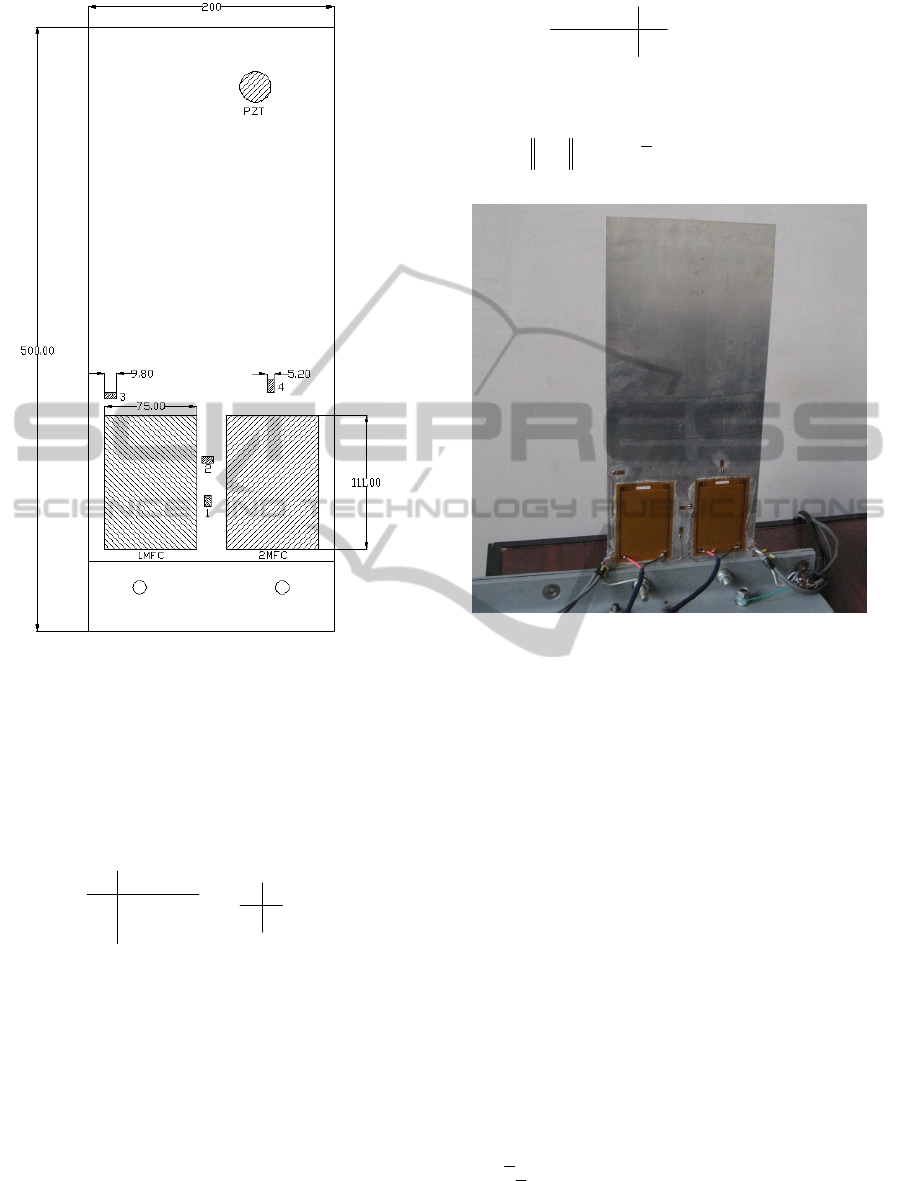
Figure 1: Sketch of the basic smart structure considered
for this study – the cantilevered aluminum plate with
bonded MFC actuators. Legend: 1MFC – the Macro Fiber
Composite (MFC) active control actuator; 2MFC – MFC
actuator for disturbance generation; 1, 1, 2, 4 – strain
gages.
The realization of the transfer matrix
(
)
Gs is
transcribed in the usual form
()
()
⎡⎤
⎡⎤
⎢⎥
⎢⎥
⎢⎥
⎢⎥
⎣⎦
⎢⎥
⎣⎦
=
12
11112
22122
-1
AB B
AB
Gs = C D D := =
CD
CD D
CsI-A B+D
(12)
These equations characterize a SISO (Single-Input-
Single-Output) system, for which an
H
∞
optimal
control problem is posed: find a controller
(
)
Ks
that
will minimize the peak value of the frequency
response of
(
)
1
zu
s
T
, the matrix-valued closed-loop
transfer function from the system input to its output
(see Fig. 4). In other words, the question is to find a
controller
(
)
Ks
()
()
:
∞
⎡
⎤
⎢
⎥
=
⎢
⎥
⎣
⎦
cc
cc
AB
Ks =
CK D
2
u
cccc
cc c
y
Dy
=+
=+
xAxB
Cx

(13)
that internally stabilizes the closed-loop system and
that, given
0γ> , satisfies the condition
()
11
R
:sup
zu zu
j
∞
ω∈
⎡⎤
=
σω<
γ
⎣⎦
TT
(14)
Figure 2: Photo of the cantilever aluminum plate specimen
performed for active control laws validation.
A justification for the optimal
H
∞
control
resides in the minimax nature of the problem, with
the argument that minimizing the “peak” of the
transfer
1
uz→ necessarily renders the magnitude
of
1
zu
T
small at all frequencies. In other words,
minimizing the
H
∞
-norm of a transfer function is
equivalent to minimizing the energy in the output
signal due to the inputs with the worst possible
frequency distribution. This improvement of the
“worst-case scenario” has a direct correspondent in
the active vibration control problem and seems
particularly attractive for light structures with
embedded piezoelectric actuators.
Before
H
∞
control synthesis can be employed,
it is necessary to verify that the open-loop plant
satisfies several assumptions (Zhou et al., 1996).
Specific desired loop gain are (Postletwhite and
Skogestad, 1993): a) for perturbation rejection
make
()
σ
KG large and b) for noise attenuation
make
()
σ
KG small (Figure 3). The specific low
frequency
l
ω
and high frequency
h
ω depend on the
specific applications.
ICINCO 2011 - 8th International Conference on Informatics in Control, Automation and Robotics
492

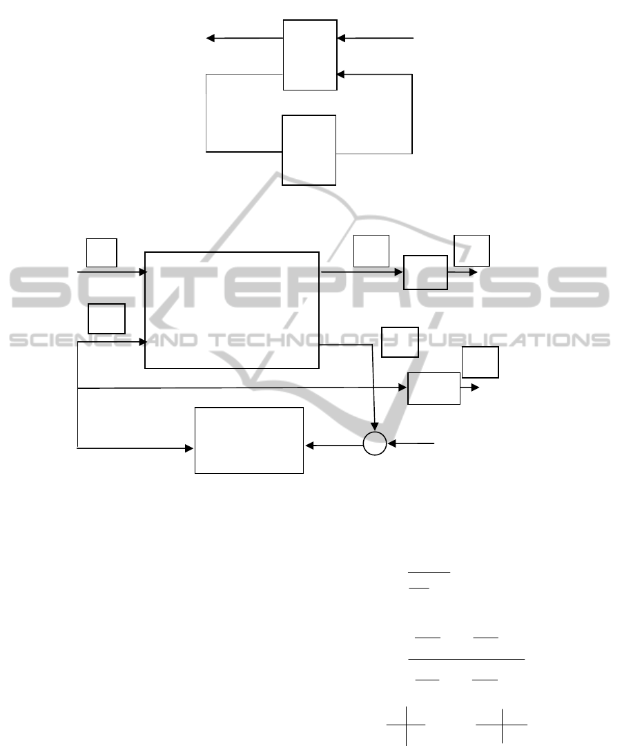
Figure 3: The
H
∞
control paradigm.
Figure 4: Block diagram of the augmented system. Dynamic weights.
We note that the observer-based
H
∞
controller (12)
is a dynamic one, even though it is based on static
weights, see the matrices
.
11221
C, D , D
3.2 Augmented System: Dynamic
Weighting Functions
The system inputs and outputs can be modified in
order to specify certain performance objectives to be
met by the closed-loop system, and to account for
the relative magnitude of the signals (Zhou et al.,
1996). Consider the system of equations (11) with
weighted regulated outputs as shown in Figure 6,
where the loop is closed by the controller
K , yet to
be determined. We denote by
η
W the diagonal
transfer matrix of first-order low pass filter,
weighting the modal coordinates in the regulated
outputs vector and by
act
W the transfer matrix of
second order band-stop filters, or first-order high-
pass filters, weighting on the piezoelectric control
voltages
,1,,,
1
1
i
i
ii
k
Win
s
k
η
η
=
=
+
ω
…
23
14
11
11
11
11
act act
act act
act act
ss
Wk
ss
⎛⎞
⎛⎞
⎜⎟
⎜⎟
++
⎜⎟
⎜⎟
ωω
⎝⎠
⎝⎠
=
⎛⎞⎛ ⎞
⎜⎟⎜ ⎟
++
⎜⎟⎜ ⎟
ωω
⎝⎠⎝ ⎠
⎡⎤
⎡⎤
⎢⎥
=
⎢⎥
⎢⎥
⎢⎥
⎣⎦
⎣⎦
ηη
act act
η act
ηη act act
AB
AB
W, W=
CD C D
(15)
The idea is to place greater emphasis on suppressing
the response due to low-frequency excitation while
avoiding a response to small high-frequency
components which will excite faster modes. Further
on, the piezo actuator signals are subject to identical
weighting functions W
act
chosen such that at
G
K
z
y
u
2
u
1
G
η
W
act
W
K
μ
w
2
u
1
z
2
z
1
e
2
e
ACTIVE ROBUST CONTROL OF A SMART PLATE
493

undesired very low and at high frequencies, herein,
the weight magnitude is increased, thus reducing the
controller response, while in the target bandwidth it
is decreased. Thus, partitioning the matrix
T
T
⎡⎤
⎣⎦
111
C:= C 0
, we can write the augmented system
(Figure 4)
,
u =
x =A x +B z =A x +B C x x =
ηηηη1 η n n 11 act
Ax+Bz=Ax+B
act act act 2 act act act 2

,
,uy =
e =C x +D z =C x +D C x e =
1 ηη η1 ηη η11 2
C x +D =C x+D w
act act act 2 2 21
2
u
y
u
⎡⎤ ⎡⎤
⎡⎤
⎢⎥ ⎢⎥
⎢⎥
⎢⎥ ⎢⎥
⎢⎥
⎢⎥ ⎢⎥
⎢⎥
⎣⎦
⎣⎦ ⎣⎦
⎡⎤
⎡⎤
⎢⎥
⎢⎥
+
⎢⎥
⎢⎥
⎢⎥
⎢⎥
⎣⎦
⎣⎦
⎡⎤
⎡⎤
⎡⎤
⎢⎥
⎢⎥
⎢⎥
⎢⎥
⎢⎥
⎢⎥
⎢⎥
⎢⎥
⎢⎥
⎣⎦
⎣⎦
⎣⎦
⎡⎤ ⎡ ⎤
⎢⎥ ⎢ ⎥
+
⎢⎥ ⎢ ⎥
⎢⎥ ⎢ ⎥
⎣⎦ ⎣ ⎦
ηη11 ηη
act act
12
12
act
η 11 η
1
2actη
2
act
1act
21
xA00x
x=BC A0x+
x000x
BB
0u+ 0
0B
DC C 0
ex
e= 0 0C x +
C00
x
00
0u+D
D0



(16)
4 LQG/LTR CONTROL
SYNTHESIS
Consider Single-Input-Single-output (SISO) system.
The LQG (Linear Quadratic Gaussian) (Kalman,
1960) control synthesis concerns the system
12
u=++xAxBfB



,
1
=zCx
,
221
yD=+μCx

(17)
and a stochastic framework which assumes the
exogenous signals

f and μ display the
characteristics of white noise signals. The goal is to
find a control
u
such that the system is stabilized
and the control minimizes the cost function
() ()
()
()
{
}
1
lim
LQG
T
J
Eu dt
u
R
T
→∞
=
⎡⎤⎡⎤
⎡⎤
⎣⎦
⎢⎥
⎢⎥
⎣⎦
⎣⎦
∫
T
T
0
Q0
xt
xt t
t
0
ρR
T
1J1
Q=C Q C, =
(18)
where
J
Q and
ρ
are weights (
ρ
is herein scalar).
The solution is given by the classical Kalman
synthesis. The state estimator has the form
()
ˆˆ ˆ
y

2f 2
x=Ax+B u+K -C x
(19)
The LQG control synthesis concerns the solving of
the decoupled algebraic Riccati equations
μ
R
0
f
−
−
−
−
=
T1TT
22 1J1
TT1 T
2211
AP+PA PB BP+CQC=0
AS + SA SC Q C S + B Q B


(20)
where

f
Q and Q
μ
are the matrices describing the
noise characteristics. The control u, the controller
gain,
c
K , the filter gain,
f
K , and the filter matrix,
respectively, are defined by,
(
)
(
)
ˆ
u
−
−
−
−−
c
1T T 1
c2f2
f
02cf2
t= Kxt
K=RBP , K=SCQ
A=A BK KC

(21)
Using the state-estimator and the control law, the
closed loop system becomes
()
() ()
21
ˆ
ˆˆ
μD
12c
f2 f 0
x(t) = Ax(t) + B f(t) - B K x t
x t = K C x(t) + K (t) + A x t




(22)
It is well known that the Linear Quadratic
Regulator (LQR) controller has good robustness
properties, but these properties are usually lost when
the LQR is used in conjunction with the Kalman
filter (Doyle, 1978). In the following, the LQG/LTR
(Loop Transfer Recovery) procedure (Stein and
Athans, 1987) will be applied to recover the lost
robustness of the LQR system. The filter gain
synthesis will be performed such that
12
D ,→0

12
B=B
(23)
and also, such that
(
)()
jj≅
LQG LQR
L ω L ω
(24)
in a certain range, as large as possible
[
]
max
0,ω∈ ω ,
where
(
)
j
s
ω
=
() ()
()
() ( )
−
−
−
−−−−
−
−−
1
LQG c f 2 2 c
1
f2 2
1
LQR c 2
Ls=KsIAKCBK
KC sI A B
Ls=KsIAB
(25)
Thus, the filter gain
f
K will be tuned so that the
closed-loop LQG/LTR system (having the open loop
matrix
LQG
L
) recovers internal stability and some of
the robustness properties (gain and phase margins)
ICINCO 2011 - 8th International Conference on Informatics in Control, Automation and Robotics
494

of the LQR design (with open loop matrix
LQR
L
).
Moreover, standard statements similar to those
already enunciated can be added: a) for perturbation
rejection
()σ
LQG
L
is to be designed large and b) for
noise attenuation
()σ
LQG
L
is to be designed small.
0 5 10 15 20 25 30 35 40 45
0
0.01
0.02
0.03
0.04
0.05
0.06
0.07
Frequency (Hz)
|Y(f)|
Figure 5: Results on cantilever plate process identification.
5 EXPERIMENTAL RESULTS ON
AN ELEMENTARY SMART
STRUCTURE
To test the proposed smart structures control
strategies,
a 200×500×1.25 mm cantilever aluminum
plate (Figures 1, 2) is considered. The test rig
contains 1) the cantilever aluminum plate on which
the strain gages (SGD-5/350-LY11, Omega
Engineering) and MFC (M8557P1MFC, Smart
Materials) actuators are bonded, 2) the signal
conditioners (OM5-WBS-3-C, Omega Engineering)
for converting strain gages bridge signals to high
level and for bridge supply, 3) the high voltage
amplifiers (PA05039,-500 V÷ +1500V) for the MFC
actuators supply, 4) a PC on which the control laws
are implemented and 5) an acquisition card (NI
PCIe-6259) used for processing the signals from
conditioners and for applying to the MFC actuator
the control signal, amplified by the high voltage
amplifiers.
The values of the matrices
122
A, B , B ,C

were
obtained by ANSYS analysis combined with
analytic considerations based on the setup of the
measured and regulated outputs. We note here that
only one of the strain gages bonded on specimen
was operational during the tests thus limiting the
experiments to a single-output case. The first five
natural frequencies of the plate identified from the
FE model are 5.66 Hz, 25.23 Hz, 33.95 Hz, 81.03
Hz, 95.05 Hz. Only a small modal damping factor of
1% of the critical damping was applied to the model.
The experimental frequencies identified with the
setup described are 5 Hz, 26 Hz, 31 Hz, 157 Hz.
Figure 5 shows the results of a simple process
identification procedure based on impulse type
perturbation. There is an acceptable match of the
first three frequencies between the model and the
measured ones. However, this does not apply for the
higher modes, with only the mode at 157 Hz being
detected by the strain gages. Consequently, only first
three modes will be taken into account in the matrix
1
C . Figure 6 presents all the system matrices
defined in (12), (13) both with the “static” weights.
The consistency of the first three modes in process is
attested by Figure 7. The frequency responses of the
weighting filters (16) are shown in Figure 8. In
choosing the dynamic weights, it is to mention the
continuity with the static weights
12 3
ηη η
k = 322, k = 39.3, k = 1.0881
−
−−
1
2
3
ω =35.6091 rad/s
ω =158.5449 rad/s
ω =213.3373 rad/s
123
2kkk===
14
23
aa
aa
ω =18.85 rad/s, ω =1885 rad/s
ω =25.13 rad/s, 0.5, ω =219.9 rad/s
act
k =
The steps of
H
∞
control synthesis, described in
Sections 3.1 and 3.2, have been validated by
numerical simulations and experiments (see Figures
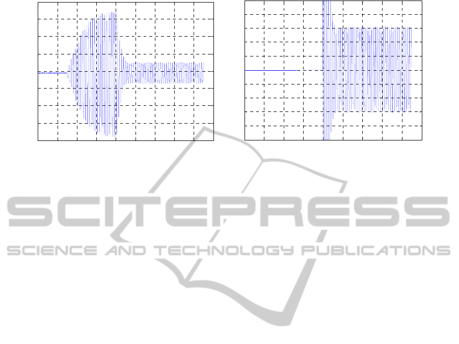
9, 10). A notable vibration attenuation of 17.4 dB is
experimentally reached (Figure 10). For the sake of
comparison, we cite the result 15.6 dB in (Yaman et
al., 2002). The simulation result predicts a
somewhat better performance, with a value of 26 dB
for the attenuation (Figure 9). The attenuation values
in the case of dynamic weights are similar. The
better attenuation predicted by the model is
explained primarily by the very small value of
damping introduced in the model, very likely
significantly smaller than the true damping value.
This essentially leads to an over-prediction of the
vibration amplitudes in the simulations.
Additionally, the actuator efficiency in the model is
considered to be ideal. A perfect actuator bonding to
the plate base structure was assumed, without any
modeling of the adhesive bond-line effects. Also, the
actuator electro-mechanic behavior was assumed to
be linear, without accounting for any hysteretic or
other nonlinear effects. Finally, we note that the
controller is derived for the numerical model, and
ACTIVE ROBUST CONTROL OF A SMART PLATE
495

thus a certain reduction in performance is to be
expected when applied to the real structure.
We emphasize now the reason for justifying the
use of an
H
∞
augmented system, instead of
nominal one. When exciting the structure at 157 Hz,
close to the fourth natural frequency, control
spillover is noticeable. The fourth mode is not
accounted for into the structural model during the
controller synthesis phase and thus susceptible to
spillover. Figure 11 exemplifies this phenomenon
for the case of closed loop control with static-
weights. However, the controller response can be
significantly reduced through weighting the
regulated output variable, as shown in Figure 12.
The application of the robust LQG/LTR control law
is exemplified in Figure 13.
6 CONCLUDING REMARKS
This paper shows how to handle the apparatus of
applied control for the problem of active vibration
control design in smart structures. Both the
theoretical background and the logistics defining the
experimental specimen are presented. Two different
approaches for the synthesis of robust control are
detailed – robust
∞
H
control and LQG/LTR
control, as comparison term. It is worth noting the
theoretical apparatus is confirmed by laboratory
tests. Dynamic weights were successfully used as a
method to prevent
∞
H control saturation. Also, the
experimental results show a comparable trend with
others reported in the literature.
55
1270 0 0 0 0 0 7122 0 0 0 0
0 25140 0 0 0 0 3 1709 0 0 0
0 0 45510 0 0 0 0 4 2667 0 0
0 0 0 259270 0 0 0 0 10 1837 0
0 0 0 0 356680 0 0 0 0 11 9445
55
.
.
.
.
.
××
⎡ ⎤
⎢ ⎥
−−
⎢ ⎥
⎢ ⎥
−−
=
⎢ ⎥
−−
⎢ ⎥
⎢ ⎥
−−
⎢ ⎥
−−
⎢ ⎥
⎣ ⎦
0I
A
51 51
1
0.0012 0
0.0012 0
0.0029 0
0.0015 0
0.0011 0
××
⎡⎤
⎢⎥
−
⎢⎥
⎢⎥
−
=
⎢⎥
−
⎢⎥
⎢⎥
−
⎢⎥
⎢⎥
⎣⎦
00
B
,
51
2
0.0012
0.0012
0.0030
0.0016
0.001
×
⎡⎤
⎢⎥
−
⎢⎥
⎢⎥
=
⎢⎥
⎢⎥
⎢⎥
⎢⎥
⎢⎥
⎣⎦
0
B
,
[
]
[]
() ( ) ()
()
2
215
38
22 2
84
21 1
18
0.0322 0.0039 0.1088 0.00878 0.0878
diag 1 , 2 , 3 0
10 0 1 , 10
0
0.5
u
CC C
×
×
−
×
=− − − − −
⎡
⎤
⎢
⎥
=
×=× ×
⎢
⎥
⎣
⎦
ρ=
C0
DC
+
56 9 7 195 2 15 5 157 366 1 0 0 0 0
10312 343 27 280410 1 000
38 7 4 7 129 4 10 4 105 6 0 0 1 0 0
18 02 62 04 5 0 0 0 1 0
24 03 83 06 67 0 0 0 0 1
4597 6 347 9 10852 1 828 0 8366 7 27 9 0 12 6 0 0
2482 7 25475
c
....
.. . . .
.. . . .
.. . .
.. . . .
A
.. . . .. .
..
−−− −−
−−− −−
−−− − −
−− − − −
−− − − −
=
−− − − −
9 87442 7520 7599 292 32 135 0 0
4642 9 483 4 60144 8 1065 5 10766 7 69 7 0 1 36 5 0 0
1316 5 115 4 3886 9 259015 8 2562 6 36 8 0 17 10 1 0
792 5 126 1 3008 4 280 2 359508 0 23 8 0 042 11 0 0 11 9
.. ...
.. . . ....
.. . . .. .
.. . . .... .
⎡ ⎤
⎢
⎢
⎢
⎢
⎢
⎢
⎢
⎢
⎢
−−− −
⎢
−−− − − − −
⎢
⎢
−−
⎢
⎢
−−− − − − −
⎣
⎥
⎥
⎥
⎥
⎥
⎥
⎥
⎥
⎥
⎥
⎥
⎥
⎥
⎥
⎦
[ ]
[]
8
0.0362 0.0064 0.0243 0.0012 0.0015 1.9225 1.7461 2.474 0.5889 0.6506
10
119.426 0.2532 231.2168 0 0 11.6708 0.0207 5.3994 0 0 ,
T
c
c
−−−−−−−− −
=×
=−
c
B
CD=0
Figure 6: The cantilever plate matrices. The system matrices defined in (12), (13) and the “static” weights.
ICINCO 2011 - 8th International Conference on Informatics in Control, Automation and Robotics
496

0 2 4 6 8 10 12 14 16 18
-5
-4
-3
-2
-1
0
1
2
3
4
5
x 10
-4
First three modes combination
t[s]
ε
y
0 2 4 6 8 10 12 14 16 18
-5
-4
-3
-2
-1
0
1
2
3
4
5
x 10
-4
All modes combination
t[s]
ε
y
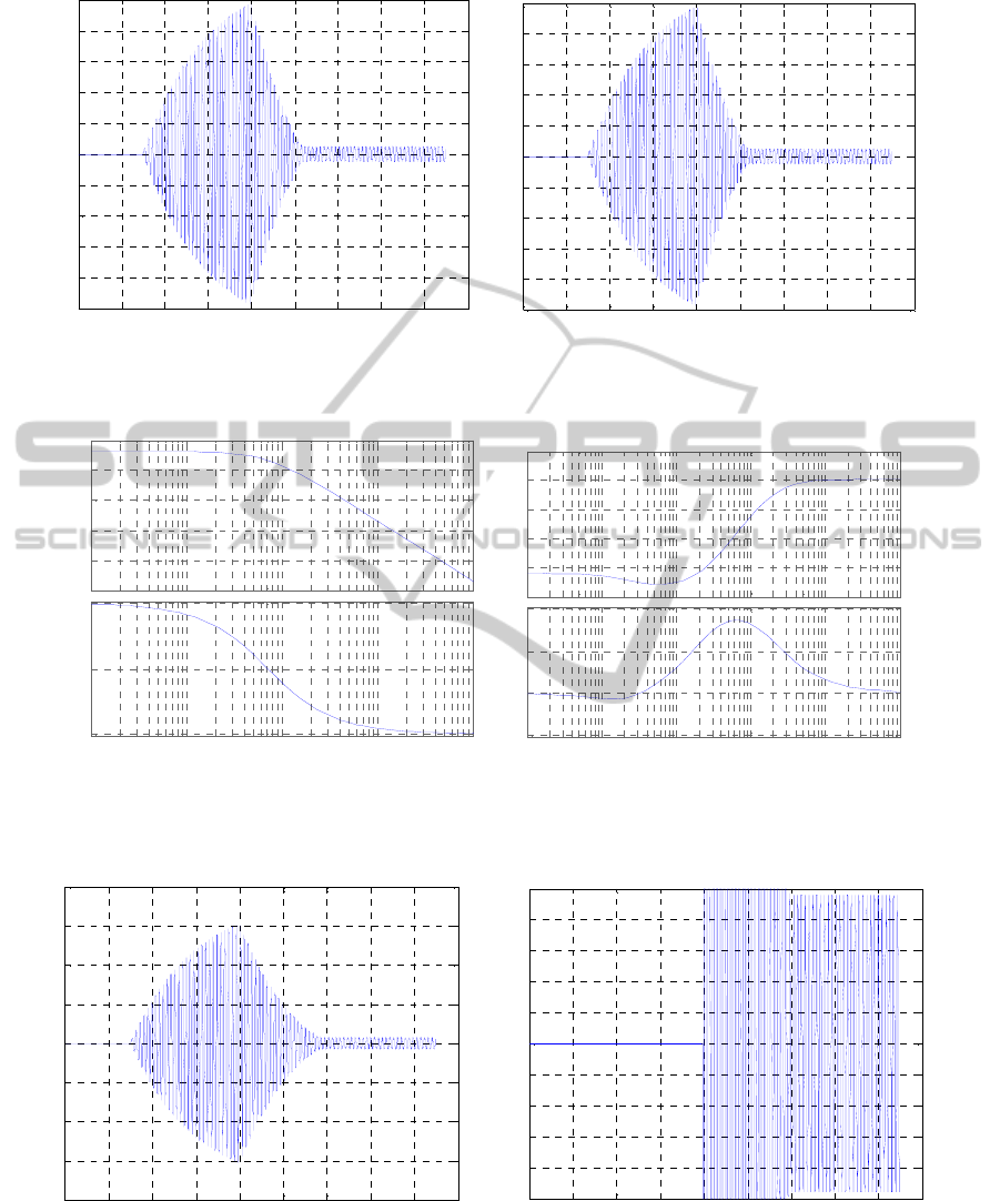
Figure 7: The consistency of the basic first three modes, static weights,

400sin 2 5.66
V
f
t
=
π×

.
-10
0
10
20
30
40
Magnitude (dB)
10
0
10
1
10
2
10
3
10
4
90
135
180
Ph
ase
(d
eg
)
Bode Diagram
Frequency (rad/sec)
-70
-65
-60
-55
-50
-45
M
agn
it
u
d
e
(dB)
10
0
10
1
10
2
10
3
10
4
10
5
-30
0
30
60
Ph
ase
(d
eg
)
Bode Diagram
Frequency (rad/sec)
a) b)
Figure 8: Weighting functions: a)
η
W , first mode; b)
act
W .
0 2 4 6 8 10 12 14 16 18
-8
-6
-4
-2
0
2
4
6
8
x 10
-4
t[s]
ε
y
Strain without and with control
0 2 4 6 8 10 12 14 16 18
-500
-400
-300
-200
-100
0
100
200
300
400
500
t[s]
u [V]
Control
Figure 9: H
∞
, static weights, numerical simulation,

500sin 2 5.66 V
f
t=π×

.
ACTIVE ROBUST CONTROL OF A SMART PLATE
497

0 2 4 6 8 10 12 14 16 18
-2
-1.5
-1
-0.5
0
0.5
1
1.5
2
2.5
x 10
-4
Strain without and with control
t[s]
ε
y
0 2 4 6 8 10 12 14 16 18
-500
-400
-300
-200
-100
0
100
200
300
400
500
C
on
t
ro
l
t[s]
u [V]
Figure 10: H
∞
, static weights, experimental record,

500sin 2 5
V
f
t=π×

.
0 2 4 6 8 10 12 14 16 18
-4
-3
-2
-1
0
1
2
3
4
5
x 10
-5
Strain without and with control
t[s]
ε
y
0 2 4 6 8 10 12 14 16 18
-200
-150
-100
-50
0
50
100
150
200
250
Control
t[s]
u
[V]
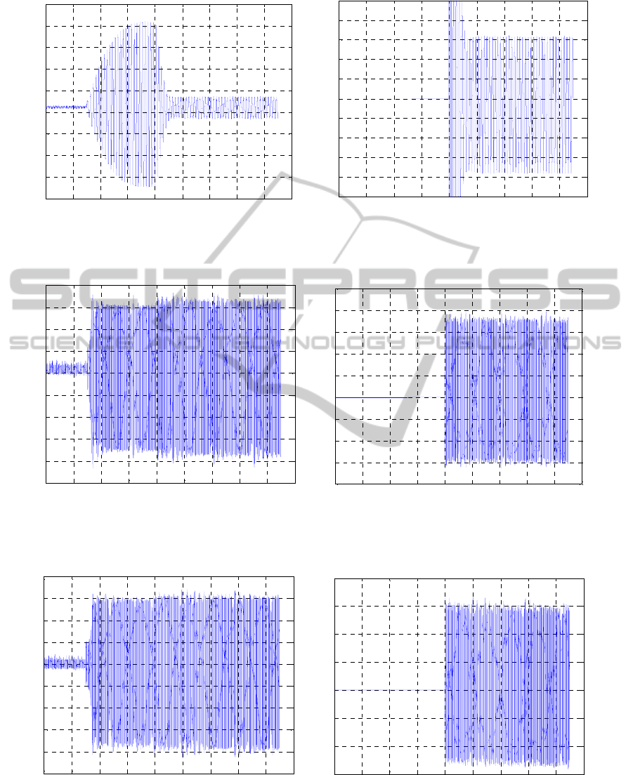
Figure 11: H
∞
, static weights, experimental record,

500sin 2 157
V
f
t=π×

.
0 2 4 6 8 10 12 14 16 18
-4
-3
-2
-1
0
1
2
3
4
5
x 10
-5
Strain without and with control
t[s]
ε
y
0 2 4 6 8 10 12 14 16 18
-150
-100
-50
0
50
100
150
200
C
on
t
ro
l
t[s]
u [V]
Figure 12: H
∞
, dynamic weights, experimental record,

500sin 2 157
V
f
t=π×

.
ICINCO 2011 - 8th International Conference on Informatics in Control, Automation and Robotics
498

0 2 4 6 8 10 12 14 16 18
-2
-1.5
-1
-0.5
0
0.5
1
1.5
2
x 10
-4
Strain without and with control
t[s]
ε
y
0 2 4 6 8 10 12 14 16 18
-500
-400
-300
-200
-100
0
100
200
300
400
500
C
ontrol
t[s]
u [V]
Figure 13: LQG/LTR, experimental record, 400sin 2 5 V
f
t=π×

.
ACKNOWLEDGEMENTS
The authors from INCAS gratefully aknowledge
the financial support of the National Authority for
Scientific Research ANCS-UEFISCSU, through
PN-II Research Project code ID 1391/2008.
REFERENCES
Doyle, J. C. (1978), Guaranteed margins for LQG
regulators,
IEEE Transaction on Automatic Control,
AC-23, 4, pp. 756-757.
Iorga, L., H. Baruh, I. Ursu (2008), A review of
H
∞
robust control of piezoelectric smart structures,
Transactions of the ASME, Applied Mechanics
Reviews
, 61, 4, July, pp. 17-31.
Iorga, L., H. Baruh, I. Ursu (2009),
H
∞
control with
μ -analysis of a piezoelectric actuated plate, Journal
of Control and Vibration
, 15, 8, pp. 1143-1171,
SAGE Publications.
Joshi, S. M., A. G. Kelkar (1998), Inner loop control for
supersonic aircraft in the presence of aeroelastic
modes,
IEEE Trans. on Control Systems Technology,
6, 6, 730-739.
Kalman, R. E. (1960), Contributions to the theory of
optimal control,
Bol. Soc. Mat. Mexicana, 5, pp.
102
−109.
Kar, N. I., T. Miyakura, K. Seto (2000), Bending and
torsional vibration control of a flexible plate
structure using based robust control law,
IEEE
Trans. on Control Systems Technology, 8, 3, pp.
545-553.
Postlethwaite, I., S. Skogestad (1993), Robust
multivariable control using
H
∞
methods: Analysis,
design and industrial applications, in
Essays on
Control – Perspectives in the Theory and its
Applications
, Birkhäuser, Boston – Basel – Berlin.
Stein, G., M. Athans (1987), The LQG/LTR procedure
for multivariable feedback control design,
IEEE
Transactions on Automatic Control
, AC-32, 2, pp.
105-114.
Yaman, Y., T. Caliskan, V. Nalbantoglu, E. Prasad, D.
Waechter (2002), Active vibration control of a smart
plate,
presented at ICAS 2002.
Ursu, I., F. Ursu (2002),
Active and semiactive control,
Romanian Academy Publishing House (in
Romanian), Bucharest.
Zhou, K., J. Doyle, K. Glover (1996),
Robust and
optimal control
, Prentice Hall, Upper Saddle River,
NJ.
ACTIVE ROBUST CONTROL OF A SMART PLATE
499